Ridiculous branching fractions nailed

B hadrons are fascinating bodies. They are bound states of a bottom quark and lighter ones, and due to the smallness of a parameter called , the element of the Cabibbo-Kobayashi-Maskawa mixing matrix, they live more than a trillionth of a second before disintegrating.

A trillionth of a second sounds like a really short lifetime, but it is not so short in the realm of particle physics, where states with lifetime millions of times shorter yet are not uncommon. A B hadron created in a high-energy collision (one of the thousand per second produced in the core of the CDF detector at Fermilab) can travel several millimeters away from the collision point before decaying.

A recent analysis by the CDF collaboration has focused on rare decays of electrically-neutral B hadrons: both mesons ( states, with q any quark lighter than the bottom) and baryons ( states, where q, q’ indicate light quarks). The searched decays were ones yielding just a pair of oppositely-charged lighter hadrons, none of which containing the next-lightest quark, the charm.

The bottom quark decays by charged current interaction, emitting a W boson and transmuting into a lighter quark. As I hinted above, the transition is usually , and its “strength” is proportional to the square of the CKM matrix element .  However, nothing prevents a direct transition to an up quark: . This process however is much less frequent, because the ratio is very small: bottom hadrons usually decay to ones containing charm.

Studying the two-body decays of a few B hadrons to states not containing charm is difficult because of the rarity of these phenomena. However, CDF is well equipped: thanks to the Silicon Vertex Tracker, a wonderful device capable of measuring track parameters in a time of about 10 microseconds,  events with two tracks not pointing back to the point where the beams cross (where the proton-antiproton collision must have originated) can be collected with high efficiency.

The power of SVT is that it not only measures track momenta -from the curvature of tracks in the magnetic field: it also can measure the track impact parameter orthogonally to the beam direction, with a precision practically identical to the one that more sophisticated, slower algorithms can obtain. Huge samples of B hadron decays are thus made available to analysis.

A recent study of CDF has used track pairs to put in evidence charmless decays of B hadrons which have really tiny branching fractions: we go from the decay , which is measured at , to the , measured at , to the , measured at . How did CDF measure such rare decays ?

The easy part is to reconstruct a mass distribution. You take the two tracks in SVT-triggered events passing an optimized data selction, and compute the track-track mass under the hypothesis that the two track are charged pions. You need to hypothesize some mass for the two bodies, which could be pions but could also be kaons or protons or other particles with lifetime long enough to leave a full track in the detector. Once you do that, you get a distribution like the one shown below (and for the moment, ignore the various colored distributions and concentrate on the black bullets with error bars):

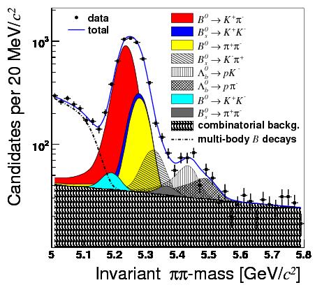
Now, the distribution of black points contains several important features. Even ignoring the various coloured areas under the points, one can see them clearly. There is an evident background right under the main peak and across all mass values, but also a nasty shoulder at low mass. Furthermore, the main peak does appear to be the composition of different contributions. It is not too hard to figure out what is the origin of the different components, however, even without reading the fine print.

First of all, the flat background, visible mainly on the right, is plausibly due to random combinations of charged tracks which do not originate from a resonance decay. The flatness of their mass spectrum is in fact a trademark of the randomness with which one may associate pairs of tracks which have nothing to share.

Then, the “shoulder” on the left. This is trickier, but you can understand what is its source if you size it up: it is something which happens more or less as frequently as two-body B hadron decays, and yet does not produce a distinct peak at the mass of the B hadron (which is of the order of 5.3 GeV), but lower. These events are due to B hadrons which produced two charged tracks, plus other particles: either charged, or neutral ones. By picking only two tracks to compute the hadron mass in these cases, one seriously underestimates the mass of the decaying object. The effect has a “turn-off” for masses just below the B hadron mass, because it becomes quite infrequent to have lost a track and still manage to reconstruct a mass quite close to the true one: even having lost a single pion would result in a negative bias of about 140 MeV.

The signal peak at the center of the graph is the composition of several different ones. Here, we must remember two things. The first is that we are observing not one single particle, but at least three: the , which has a mass of 5.279 GeV; the , which is a meson containing a bottom and a strange quark in a combination, and weighs 5.367 GeV; and the , which is a baryon and weighs 5.620 GeV. So the “bump” is indeed the combination of three particle decays. But also important to remember is that we arbitrarily assigned the mass of the charged pion (0.139 GeV) to the two tracks! In a two-body decay of a B hadron not only pions, but also kaons and protons are produced: and since the masses of the latter particles are quite a bit larger than that of pions (respectively, 0.495 and 0.938 GeV), we underestimate appreciably the hadron mass when we reconstruct it that way!

I am sure I have managed to confuse most of you. What is the rationale, I can hear you mutter, of assuming the pion mass for tracks that are not pions ? Well: look at the plot! If we reconstructed all mesons at the true mass, we would be unable to tell the different decays of these mesons apart, because they would all peak in a very similar fashion at the same mass: we would lose the discriminating power of the reconstructed mass, the variable we are plotting. And besides: CDF cannot easily discriminate pions from kaons and protons, so we are somehow forced to make an assumption. The “minimal” one is the one which is used in such cases.

If you give another critical look at the plot, knowing now why the different decays are expected to produce peaks at different “track-track” mass values, you may well raise an eyebrow: there are eight different components contributing to the central structure, and the data points cannot certainly discriminate them all! How can CDF claim to be measuring each of those decays so precisely ?

Well, first of all, not all of those components are determined with precision: the two smaller ones, the and , are not determined by the CDF analysis (CDF only puts a 90%CL limit on their cross section, in fact).  But of course, there is one missing piece in the puzzle, which I have so far hidden from your view. It is the track ionization measurement.

Charged tracks ionize the gas filling the CDF tracking chamber at different rates per unit distance traversed, depending on their speed. We measure the momentum of tracks from their curvature in the magnetic field, but momentum is speed times mass. By determining the amount of charge that is freed by the gas atoms along the particle path, we have a handle to discriminate different ones, combining that information with the particle momentum. See the graph below:

In the graph -admittedly, a very complicated one-, you can see how different particles carrying the same momentum exhibit a different energy loss. On the horizontal axis you have the particle momentum in GeV units, on the vertical axis the amount of energy loss per unit distance they exhibit. Each detected particle is a small black dot in the graph, and you immediately see that the dots cluster along different lines. These lines -which are rather more like bands, since there is some uncertainty in the quantities plotted- characterize the different behavior of each particle. You see that the same behavior -a rapidly falling curve, followed by a slow rise for very high momenta- is repeated for the different particles at different values of momentum, because different particles have different masses, and the ionization loss only depends on speed, not momentum. (For electrons the functional dependence is different, but that is another story, worth a separate post…)

Now, to make an example: say you have a 0.7 GeV/c track and you measure a ionization of 2 “units” (the quantity on the Y axis). After checking the plot above, you can be reasonably sure it is a proton, if your ionization and momentum measurements are any good. In fact, the discrimination is not very efficient, because CDF can only measure ionization with low resolution, by the width of electronic pulses on the wires collecting the charge.

Now, let us go back to the problem of discriminating different B hadron decays. Each of the two tracks in these events is classified based on their measured ionization, and the information is used in a likelihood function. Another likelihood function incorporates all the information on the kinematics of the two particles, and the product of these functions is used to discriminate the different decays. In the end, the mass distribution you saw above displays the result of the fit, where the different components are fixed by not just their mass values, but by all the kinematic and energy loss information each event possesses.

Knowing the level of detail of the analysis which lies behind the measurement, I am impressed by the accuracy with which these rare decays have been nailed by CDF, and I do not hide the fact that it makes me proud to sign the paper which I finished reviewing today, and is just about to be sent to PRL. But, there remains a question. Now that we know these branching fractions so precisely, what do we do with them ?

Of course: we add a line to the PDG data book! But seriously, there are implications for new physics theories. Indeed, some of these decays are predicted to be larger by Supersymmetric theories with R-parity violation. So, these measurements are yet another small step in the same direction: kicking SUSY out of the table, bit by bit. It will take a while, though!