Things I should have blogged on last week April 13, 2009
Posted by dorigo in cosmology, news, physics, science.Tags: anomalous muons, CDF, dark matter, DZERO, Higgs boson, neutrino
comments closed
It rarely happens that four days pass without a new post on this site, but it is never because of the lack of things to report on: the world of experimental particle physics is wonderfully active and always entertaining. Usually hiatuses are due to a bout of laziness on my part. In this case, I can blame Vodafone, the provider of the wireless internet service I use when I am on vacation. From Padola (the place in the eastern italian Alps where I spent the last few days) the service is horrible, and I sometimes lack the patience to find the moment of outburst when bytes flow freely.
Things I would have wanted to blog on during these days include:
- The document describing the DZERO search of a CDF-like anomalous muon signal is finally public, about two weeks after the talk which announced the results at Moriond. Having had in my hands a unauthorized draft, I have a chance of comparing the polished with the unpolished version… Should be fun, but unfortunately unbloggable, since I owe some respect to my colleagues in DZERO. Still, the many issues I raised after the Moriond seminar should be discussed in light of an official document.
- DZERO also produced a very interesting search for
production. This is the associated production of a Higgs boson and a pair of top quarks, a process whose rate is made significant by the large coupling of top quarks and Higgs bosons, by virtue of the large top quark mass. By searching for a top-antitop signature and the associated Higgs boson decay to a pair of b-quark jets, one can investigate the existence of Higgs bosons in the mass range where the
decay is most frequent -i.e., the region where all indirect evidence puts it. However, tth production is invisible at the Tevatron, and very hard at the LHC, so the DZERO search is really just a check that there is nothing sticking out which we have missed by just forgetting to look there. In any case, the signature is extremely rich and interesting to study (I had a PhD doing this for CMS a couple of years ago), thus my interest.
- I am still sitting on my notes for Day 4 of the NEUTEL2009 conference in Venice, which included a few interesting talks on gravitational waves, CMB anisotropies, the PAMELA results, and a talk by Marco Cirelli on dark matter searches. With some effort, I should be able to organize these notes in a post in a few days.
- And new beautiful physics results are coming out of CDF. I cannot anticipate much, but I assure you there will be much to read about in the forthcoming weeks!
Milind Diwan: recent MINOS results April 8, 2009
Posted by dorigo in news, physics, science.Tags: minos, neutrino, neutrino experiments, neutrino oscillations, Sterile neutrinos
comments closed
I offer below another piece of the notes I took at the NEUTEL09 conference in Venice last month. For the slides of the talk reported here, see the conference site.
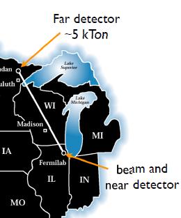 Milind’s presentation concentrated on results of muon-neutrino to electron-neutrino conversions. Minos is a “Main-Injecor Neutrino Oscillation Search”. It is a long-baseline experiment: the beam from the Main injector, Fermilab’s high-intensity source of protons feeding the Tevatron accelerator, can be sent from Batavia (IL) 735km away to the Soudan mine in Minnesota. There are actually two detectors, a near and a far detector: this is the unique feature of MINOS. The spectra collected at the two sites are compared to measure muon neutrino disappearance and appearance. The near detector is 1km away from the target.
The beam is a horn-focused muon-neutrino one. Horns are parabolic-shaped magnets. 120 GeV protons originate pions, which are focused by these structures; negative ones are defocused, and the beam contains predominantly muon neutrinos from the decay of these pions. The accelerator provides 10-microsecond pulses every 2.2 seconds, with 


Besides the presence of two detectors in line, another unique feature of the Fermilab beam is the possibility to move the target in and out, shifting the spectrum of neutrinos that come out, because the focal point of the horns changes. Two positions of the target are used, corresponding to two beam configurations. In the high-energy configuration one can get a beam centered at an energy of 8 GeV or so, while the low-energy configuration is centered at 3 GeV. Most of the time Minos runs with the 3 GeV beam.
Detectors are a kiloton-worth of steel and scintillator planes in the near detector, and 5.4-kT in the far detector. Scintillator strips are 1 cm thick, 4.1 cm wide, and their Moliere radius is of 3.7cm. A 1-GeV muon crosses 27 planes. The iron in the detectors is magnetized with a 1 Tesla magnetic field.
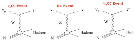
Minos event topologies include CC-like and NC-like events. A charged-current (CC) event gives a muon plus hadrons: a long charged track from the muon, which is easy to find. A neutral current (NC) event will make a splash and it is diffuse, since all one sees is the signal from the disgregation of the target nucleus; an electron CC event will leave a dense, short shower, with a typical electromagnetic shower profile. The three processes giving rise to the observed signatures are described by the Feynman diagrams below.
The analysis challenge is to put together a selection algorithm capable of rejecting backgrounds and select CC 
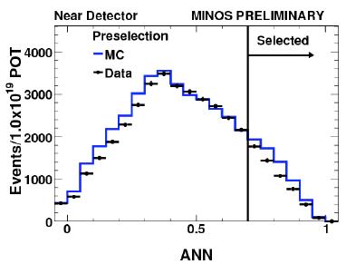
Basic cuts are applied on their data sample to ensure data quality. Fiducial volume cuts provide rejection to cosmic ray backgrounds. Simple cuts lead to a S/N ratio of 1:12. By “signal” one means the appearance of electron neutrinos.
They can select
[As I was taking these notes, I observed that data and Monte Carlo simulation do not match well in the low-ANN output region. The speaker claims tha the fraction of events in the tail of the Monte Carlo distribution can be modeled only with some approximation, but that they do not need to model that region too well for their result. However, it looks as if the discrepancy between data and MC not well understood. Please refer to the graph shown below, which shows the NN output in data and simulation at a preselection level.]
Back to the presentation. To obtain a result, the calculation they performis simple: how many events are expected in the far detector ? The ratio of far to near flux is known, 1.3E-6. This includes all geometrical factors. For this analysis they have 3E20 protons on target. They expect 27 events for the ANN selection, and 22 for the LEM analysis.
They need to separate backgrounds in NC and CC, so they do a trick: they take data in two different beam configurations, then they look at the spectrum in the near detector, where they expect muon-type events to be rejected much more easily because they are more deflected. From this they can separate the two contributions.
Their final result for the predicted number of electron-induced CC events is 27+-5 (stat)+-2 (syst).
A second check on the background calculation consists in removing the muon in tagged CC events, and use these for two different calculations. One is an independent background calculation: they can add a simulated electron to the event raw data after removing the muon. This checks whether the signal is modeled correctly. From these studies they conclude that the signal is modeled well.
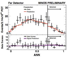
The results show that there is indeed a small signal: they observe 35 events, when they expect 27, in the high-NN output region, as shown in the figure above. For the other method, LEM, results are consistent. The energy spectrum of the selected events is shown in the graph below.

With the observation of this small excess (which is compatible with predictions), a confidence level is set in the plane of the two parameters 


 The speaker claims that if the excess they are observing disappears with further accumulated data, they will be able to reach below the existing bound.
The other result of MINOS is a 
neutrinos is less than 0.68 at 90%CL.
NeuTel 09: Oscar Blanch Bigas, update on Auger limits on the diffuse flux of neutrinos April 3, 2009
Posted by dorigo in astronomy, cosmology, news, physics, science.Tags: auger, cosmic rays, GKZ, neutrino
comments closed
With this post I continue the series of short reports on the talks I heard at the Neutrino Telescopes 2009 conference, held three weeks ago in Venice.
The Pierre Auger Observatory is a huge (3000 km^2) hybrid detector of ultra-energetic cosmic rays -that means ones having an energy above 10^18 eV. The detector is located in Malargue, Argentina, at 1400m above sea level.
There are four six-eyed fluorescent detectors: when the shower of particles created by a very energetic primary cosmic ray develops in the atmosphere, it excites nitrogen atoms which emit energy in fluorescent light, collected in telescope. It is a calorimetric measurement of the shower, since the number of particles in the shower gives a measurement of the energy of the incident primary particle.
The main problem of the fluorescent detection method is statistics: fluorescent detectors have a reduced duty cycle because they can only observe in moonless nights. That amounts to a 10% duty cycle. So these are complemented by a surface detector, which has a 100% duty cycle.
The surface detector is composed by water Cherenkov detectors on the ground, which can detect light with PMT tubes. The signal is sampled as a function of distance from the center of shower. The measurement depends on a Monte Carlo simulation, so there are some systematic uncertainties present in the method.

The assembly includes 1600 surface detectors (red points), surrounded by four fluorescence detectors (shown by green lines in the map above). These study the high-energy cosmics, their spectra, their arrival direction, and their composition. The detector has some sensitivity to unidentified ultra-high energy neutrinos. A standard cosmic ray interacts at the top of atmosphere, and yields an extensive air shower which has an electromagnetic component developing on the ground; but if the arrival direction of the primary is tilted with respect to the vertical, the e.m. component is absorbed when it arrives on the ground, so it contains only muons. For neutrinos, which can penetrate deep in the atmosphere before interacting, the shower will instead have a significant e.m. component regardless of the angle of incidence.
The “footprint” is the pattern of firing detectors on the ground. It encodes information on the angle of incidence. For tilted showers, the presence of an e.m. component is strong indication of neutrino shower. An elongated footprint and a wide time structure of signal is seen for tilted showers.
There is a second method to detect neutrinos. This is based on the so-called “skimming neutrinos“: the Earth-skimming mechanism occurs when neutrinos interact in the Earth, producing a charged lepton via charged current interaction. The lepton produces a shower that can be detected above the ground. This channel has better sensitivity than neutrinos interacting in the atmosphere. It can be used for tau neutrinos, due to early tau decay in the atmosphere. The distance of interaction for a muon neutrino is 500 km, for a tau neutrino is 50 km. for electrons it is 10 km. These figures apply to 1 EeV primaries. If you are unfamiliar with these ultra-high energies, 1 Eev = 1000 PeV = 1,000,000 TeV: this is roughly equivalent to the energy drawn in a second by a handful of LEDs.
Showers induced by emerging tau leptons start close to the detector, and are very inclined. So one asks for an elongated footprint, and a shower moving at the speed of light using the available timing information. The background to such a signature is of the order of one event every 10 years. The most important drawback of Earth-skimming neutrinos is the large systematic uncertainty associated with the measurement.
Ideally, one would like to produce a neutrino spectrum or an energy-dependent limit on the flux, but no energy reconstruction is available. Observed energy depends on the height at which the shower is developing, and since this is not known for penetrating particles as neutrinos, one can only give a flux limit for them. The limit is in the range of energy where GZK neutrinos should peak, but its value is an order of magnitude above the expected flux of GZK neutrinos. A differential limit in energy is much worse in reach.
The figure below shows the result for the integrated flux of neutrinos obtained by the Pierre Auger observatory in 2008 (red line), compared with other limits and with expectations for GKZ neutrinos.

Neutrino telescopes 2009: Steve King, Neutrino Mass Models April 2, 2009
Posted by dorigo in news, physics, science.Tags: conferences, extra dimensions, neutrino, standard model
comments closed
This post and the few ones that will follow are for experts only, and I apologize in advance to those of you who do not have a background in particle physics: I will resume more down-to-earth discussions of physics very soon. Below, a short writeup is offered of Steve King’s talk, which I listened to during day three of the “Neutrino Telescopes” conference in Venice, three weeks ago. Any mistake in these writeups is totally my own fault. The slides of all talks, including the one reported here, have been made available at the conference site.
 Most of the talk focused on a decision tree for neutrino mass models. This is some kind of flow diagram to decide -better, decode- the nature of neutrinos and their role in particle physics.
In the Standard Model there are no right-handed neutrinos, only Higgs doublets of the symmetry group 
The decision tree starts with the question: is the LSND result true or false ? if it is true, then are neutrinos sterile or CPT-Violating ? Otherwise, if the LSND result is false, one must decide whether neutrinos are Dirac or Majorana particles. If they are Dirac particles, they point to extra dimensions, while if they are Majorana ones, this brings to several consequences, tri-bimaximal mixing among them.
So, to start with the beginning: Is LSND true or false ? MiniBoone does not support the LSND result but it does support three neutrinos mixing. LSND is assumed false in this talk. So one then has to answer the question, are then neutrinos Dirac or Majorana ? Depending on that you can write down masses of different kinds in the Lagrangian. Majorana ones violate lepton number and separately the three of them. Dirac masses couple L-handed antineutrinos to R-handed neutrinos. In this case the neutrino is not equal to the antineutrino.
The first possibility is that the neutrinos are Dirac particles. This raises interesting questions: they must have very small Yukawa coupling. The Higgs Vacuum Expectation Value is about 175 GeV, and the Yukawa coupling is 3E-6 for electrons: this is already quite small. If we do the same with neutrinos, the Yukawa coupling must be of the order of 10^-12 for an electron neutrino mass of 0.2 eV. This raises the question of why this is so small.
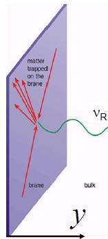 One possibility then is provided by theories with extra dimensions: first one may consider flat extra dimensions, with right-handed neutrinos in the bulk (see graph on the right). These particles live in the bulk, whereas we are trapped in a brane. When we write a Yukawa term for neutrinos we get a volume suppression, corresponding to the spread of the wavefunction outside of our world. It goes as one over the square root of the volume, so if the string scale is smaller than the Planck scale (
The other sort of extra dimensions (see below) are the warped ones, with the standard model sitting in the bulk. The wavefunction of the Higgs overlaps with fermions, and this gives exponentially suppressed Dirac masses, depending on the fermion profiles. Because electrons and muons peak in the Planck brane while we live in the TeV brane, where the top quark peaks, this provides a natural way of giving a hierarchy to particle masses.
 Some of these models address the problem of dark energy in the Universe. Neutrino telescopes studying neutrinos from Gamma-ray bursts may shed light on this issue along with Quantum Gravity and neutrino mass. The time delay relative to low-energy photons as a function of redshift can be studied against the energy of neutrinos. The function lines are different, and they depend on the models of dark energy. The point is that by studying neutrinos from gamma-ray bursts, one
has a handle to measure dark energy.
Now let us go back to the second possibility: namely, that neutrinos are Majorana particles. In this case you have two choices: a renormalizable operator with a Higgs triplet, and a non-renormalizable operator with a lepton violation term, 
We can concentrate on see-saw mechanisms in the rest of the talk. There are several types of such models, type I is essentially exchanging a heavy right-handed neutrino in the s-channel with the Higgs. Type II is instead when you exchange something in the t-channel, this could be a heavy Higgs triplet, and this would also give a suppressed mass.
The two types of see-saw types can work together. One may think of a unit matrix coming from a type-II see-saw, with the mass splittings and mixings coming from the type-I contribution. In this case the type II would render the neutrinoless double beta decay observable.
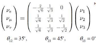 Moving down the decision tree, we come to the question of whether we have precise tri-bimaximal mixing (TBM). The matrix (see figure on the right) corresponds to angles of the standard parametrization,


Let us consider the form of the neutrino mass matrix assuming the correctness of the TBM matrix. We can derive what the mass matrix is by multiplying it by the mixing matrix. It has three terms, one proportional to mass 


Such a mass matrix is called “form-diagonalizable” since it is diagonalized by the TBM matrix for all values of a,b,d. A,b,d translate into the masses. There is no cancelation of parameters involved, and the whole thing is extremely elegant. This suggests something called “form dominance”, a mechanism to achieve a form-diagonalizable effective neutrino mass matrix from the type-I see-saw. Working in the diagonal MRR basis, if 
Moving on to symmetries, clearly, the TBM matrix suggests some family symmetry. This is badly broken in the charged lepton sector, so one can write explicitly what the Lagrangian is, and the neutrino Majorana matrix respects the muon-tauon interchange, whereas the charged matrix does not. So this is an example of a symmetry working in one way but not in the other. To achieve different symmetries in the neutrino and charged lepton sectors we need to align the Higgs fields which break the family symmetry (called flavons) along different symmetry-preserving directions (called vacuum alignment). We need to have a triplet of flavons which breaks the A4 symmetry.
A4 see-saw models satisfy form dominance. There are two models. Both have R=1. These models are economical, they involve only two flavons. A4 is economical: yet, one must assume that there are some cancelations of the vacuum expectation values in order to achieve consistency with experimental measurements of atmospheric and solar mixing. This suggests a “natural form dominance”, less economical but involving no cancelations. A different flavon is associated to each neutrino mass. An extension is “constrained sequential dominance”, which is a special case, which supplies strongly hierarchical neutrino masses.
As far as family symmetry is concerned, the idea is that there are two symmetries, two family groups from the group 


The conclusions are that neutrino masses and mixing require new physics beyond the Standard Model. There are many roads for model building, but their answers to key experimental questions will provide the signposts. If TMB is accurately realized, this may imply a new symmetry of nature: a family symmetry, broken by flavons. The whole package is a very attractive scheme, sum rules underline the importance of showing that the deviations from TBM are non-zero. Neutrino telescopes may provide a window into neutrino mass, quantum gravity and dark energy.
After the talk, there were a few questions from the audience.
Q: although true that MiniBoone is not consistent with LSND in a simple 2-neutrino mixing model, in more complex models the two experiments may be consistent. King agrees.
Q: The form dominance scenario in some sense would not apply to the quark sector. It seems it is independent of A4. King’s answer: form dominance is a general framework for achieving form-diagonalizable elements starting from the see-saw mechanism. This includes the A4 model as an example, but does not restricts to it. There are a large class of models in this framework.
Q: So it is not specific enough to extend to the quark sector ? King: form dominance is all about the see-saw mechanism.
Q: So, cannot we extend this to symmetries like T’ which involve the quarks ? King: the answer is yes. Because of time this was only flashed in the talk. It is a very good talk to do by itself.
Neutrino Telescopes Day 1 note March 11, 2009
Posted by dorigo in cosmology, news, physics, science.Tags: Borexino, Kamland, neutrino, neutrino oscillation, neutrino telescopes, proton decay, SNO, sun, Superkamiokande
comments closed
Below are some notes I collected today during the first day of the “Neutrino Telescopes” conference in Venice. I have to warn you, dear readers, that my superficial knowledge of most of the topics discussed today makes it very likely to certain that I have inserted some inaccuracy, or even blatant mistakes, in this summary. I am totally responsible for the mistakes, and I apologize in advance for whatever I have failed to report correctly. Also, please note that because of the technical nature of this conference, and the specialized nature of the talks, I have decided to not even try to simplify the material: this is thus only useful for experts.
In general, the conference is always a pleasure to attend. The venue, Palazzo Franchetti, is located on the Canal Grande in Venice. To top that, today was a very nice and sunny day. I skipped the first few “commemorative” talks, and lazily walked to the conference hall in time for coffee break. The notes I took refer to only some of the talks, those which I managed to follow closely.
Art Mc Donald, SNO and the new SNOLAB

This was a discussion of the SNO experiment and a description of the new telescopes that will start to operate in the expansion of the SNO laboratory. SNO is an acrylic vessel, 12m in diameter, containing 1000 tonnes of deuterium (
The detector is located deep underground, in the Creighton mine near Sudbury, Ontario, Canada. The depth makes for smaller cosmic-ray backgrounds than other neutrino detectors, at a depth where muons from neutrino interactions start to compete with primary ones.
SNO was designed to observe neutrinos in three different reactions:
- In the charged-current weak interaction of a neutrino with a deuterium nucleus the neutrino becomes an electron, emitting a W boson which turns the nucleus into a pair of protons. This reaction has a energy threshold of 1.4 MeV, and the electron can be measured by the Cherenkov light it yields in the liquid.
- Neutral-current interactions -where the neutrinos interact with matter by exchanging virtual Z bosons, are possible with all kinds of neutrinos, and they provide a signature of a neutron and a proton freed from the nucleus, if the incoming neutrino has an energy above 2.2 MeV.
- Finally, elastic scattering both in water and deuterium can occur between neutrinos and the electrons of the medium.
SNO tries three neutron detection methods, which are “systematically different”: they rely on different physical processes and have thus different measurement systematics. First of all, in pure heavy water one can detect neutrons by capturing them into deuterium, with the emission of a 6.25 MeV photon.
Putting salt in the detector allows to get more gamma rays from neutron capture, because the sodium chloride allow neutron capture in 35Cl, and neutral current events can be separated from charged-current events using event isotropy.
In phase III they put in an array of long tubes of ultrapure Helium-3, and observe neutron capture and measure neutral current rates with an entirely different detection system.
Measurements showed that CC and NC reactions were not the same, fluxes were in a ratio of 
Phase III consists in inserting 40 strings on a 1-meter spaced grid in the vessel, for a total of 440 meters of proportional counters filled with 3He. The signal collected in phase III amounts to 983+-77 events.
Combined with the results of the KamLAND and Borexino experiments, the fit to SNO data constrains the angle 

The future for SNO is to have it filled with liquid scintillator doped with Neodimium for double beta decay studies. 150-Nd is one of the most favourable candidates for double beta, with large phase space due to its high endpoint energy (3.37 MeV). It provides for a long attenuation length, and it is stable for more than 2 years. For double beta decays they expect to get to 0.1 eV sensitivity with a 1000 ton-mass detector.
Atsuto discussed the history and the results of the KamLand experiment. There was a first proposal of the detector in 1994, a full budget approval in 1997 by the Japanese. In April 1998 the construction started, and in 1999 US-Kamland was approved by DOE. Data taking began in 2002. In August 2009 there will be a new budget proposal, for double beta decay studies.
Kamland consists in a Xenon-filled vessel, with an outside one filled with Gadolinium. Kamland wants detects neutrino oscillation with >100 Km baseline, exploiting the many nuclear reactors in Japan. The second goal is to search for geo-neutrinos: these are potential anti-neutrinos coming from fusion processes which could hypothetically take place at the center of the Earth.
Many reactors provide the source of neutrinos, a total of 70GW (12% of global nuclear power) at an average 175+-35 km distance from KamLAND. The largest systematic for reactor neutrino detection come from the knowledge of the fiducial volume (4.7%), the energy threshold (2.3%), the antineutrino spectrum (2.5%), for a total of 6.5%.
The experiment observed neutrino disappearance, measured the parameters of neutrino oscillations, and also put an upper limit of 6.4 TW for geo-neutrinos. Theoretical models, which predict the power at 3 TW, have not been excluded yet.
Gianluigi Fogli: SNO, KamLAND and neutrino oscillations: theta_13.
Gianluigi started his talk with a flash-back: four slides which were shown at NO-VE 2008, the former instantiation of this conference. This came after the KamLAND 08 release, but before the SNO 2008 release of results.
What one would like to know is the hierarchy (normal or inverted), the CP asymmetry in the neutrino sector, and the 

In the second slide from 2008, the reason was discussed. A disagreement comes from the difference between solar data, SNO-dominated, and the kamLAND data at 

The content of Fogli’s talk was organized as a time-table of eight events, in two acts.
First: in May 2008 the effect was discussed independently by Balantekin and Yilmaz. Then, in May, SNO-III data was released. In June, our analysis giving 
Concerning atmospheric and long-baseline neutrinos, there were results yielding 0.016+-0.010 from all data in our analysis, then comments on the atmospheric hint by Maltoni and Shwetz, then a new three-flavor atmospheric analysis from SK. Finally, just a month ago we saw the first MINOS results on electron neutrino appearance.
Act one: solar and kamland hint for 

Event 3: the hints of theta_13>0 from the global analysis. We have the hint plotted in the plane of the two mixing angles, and you see that the solar and Kamland region in sintheta_13 vs sintheta_12. the agreement is reached only if 


Complementarity: solar and kamland data taken separately prefer theta_13=0. Combined they are 1.2 sigma away from zero.
Event 4 in the list given above was the analysis by Schwetz and Tortola and Valle: they also found a preference for
In conclusion, a weak preference for
The complication comes out in Act 2: event 5 is the older but persisting hint for
The excess is given by a formula,


We have two kinds of matter effects that take place in the propagation. If one assumes a constant density approximation, and with a normal hierarchy, the three quantities can be given, where one can distinguish the theta_13, the delta_m, and the interference terms. All three effects can singularly dominate. The different terms help fitting the small electron excess in sub-Gev and multi-Gev data.
The atmospheric three-neutrino analyses by the SK Collaboration (in hep-ex/0604011) and Schwetz, Tortola, and Valle in 0808.2016 cannot directly compare with the one of Fogli, because they do not include the two sub-leading solar terms, since they make the assumption of one-mass-scale-dominance.
Sticking to his own analysis, Fogli continued by taking the two hints from solar+kamland results on one side, and atmospheric neutrinos+chooz+lbl on the other: they indicate a 1.6 sigma discrepancy from zero of theta_13. Combining all data together, 

Event 6: rather recent, in December of last year Maltoni and schwetz published 0812.3161, which includes the discussion of the preliminary Superkamiokande-II data. Using SK-I data they find at most 0.5 sigma from atmospheric neutrinos plus chooz data. This is weaker than Fogli’s 0.9 sigma, but shows similar qualitative features.
Event 7: a discussion of the data of SK-I, SK-II, and maybe SK-III, even if all these things are not yet published. There eists ongoing three-flavor analyses as reported in recent PhD theses using SK I+II data. Wendell, Takenaga. Unfortunately, none of the above analyses allows both theta_13 and 
Concerning the sub-Gev electron excess, effects persist in phases I and II, but slight excess present of upgoing multi-Gev evens is present in SK I but not in SK II. This downward fluctution may disfavor a non-zero value of theta_13, as noted by Maltoni and Schwetz.
From SK-III two distributions presented at neutrino 2008 by J.Raaf show that a slight excess of upgoing multi-Gev seems to be back, together with a persisting excess of sub-Gev data.
So the question is: SK-III shows both effects. Can this be interpreted away from statistical fluctuations ? This requires a refined statistical analysis with a complete set of data coming from SuperKamiokande.
Currently, there is an impressive number of bins in energy and angle, and 66 sources of systematics. These need to be handled carefully. Such a level of refinement is difficult to reproduce outside of the collaboration, In other words, independent analyses of atmospheric data searching for small effects at the level of 1-sigma are harder to perform now. So, it will be important to see the next official SK data release and especially the SK oscillation analysis, hopefully including a complete treatment of three flavor oscillation withboth parameters allowed to go larger than 0.
In the meantime, Fogli noted that he does not have compelling reasons to revise his 0.9-sigma hint of theta_13 coming from published SK-I data.
Finally, Event 8: this last one is very recent, concerns the first MINOS results on electron-neutrino appearance. These preliminary results have been released too recently, and it would be unfair to anticipate results and slides that will be shown later in this workshop, but
Fogli could not help noticing that the MINOS best fit for theta_13 sits around the chooz limit, and is away from zero at 90% C.L.
If we see the glass half-full, then we might have two independent 90% C.L. hints in favor of theta_13>0: one coming from Fogli’s global analysis of 2008, and one coming from MINOS, that can be roughly symmetrized and approximated in the form 
 Borexino is a liquid scintillator detector. The active volume is filled by 270 liters of liquid scintillator contained in a thin nylon vessel. Light emitted is seen by Photomultiplier tubes. The outer volume is filled by the same organic material, but with a quencher in the buffer region. Water used as shield. The tubes are looking at Cherenkov light. Used for active muon veto. Borexino is a simple detector, but in practice the requirements needed for the radiopurity are tough to comply with.
The physics goals are a measurement in real time of flux and spectrum of solar neutrinos in MeV or sub-MeV range. Why measure solar neutrinos of low energy ? The LMA-MSW model predicts a specific behavior for the neutrino survival probability for the various types of neutrinos emitted in the sun. The shape of the prediction as a function of energy shows a larger survival probability at lower energy.
All data before Borexino measured higher energy. So Borexino wants to measure shape of survival probability as a function of energy, going lower. Measurement can constrain additional oscillation models. If we asssume that neutrinos oscillate and we take data of the survival probability, we get the absolute neutrino flux, and we might be able to measure the component of the CNO source in the neutrino flux, this can help constrain the solar models.
Borexino can also see antineutrinos (geo-nu), in gran sasso this will be relatively easy because background from reactor antineutrinos is small. We need statistics, several years to collect significant data. The signal to noise ratio provided by the apparatus is of 1.2. The detector has also sensitivity to supernova neutrinos. Borexino is thus entering the SNEW community.
Results of Borexino will be complementary to others. Taking data since mid march 2007. They have about 450 days of live time so far. The process of neutrino detection is elastic scattering on electrons. High scintillator yield of 500 photoelectrons per MeV, a high energy resolution, and a low threshold. No information on the direction of neutrinos, however. Scintillator is fast, can reconstruct the position with time measurements. Different answers to alpha and beta particles can distinguish the two. The shape of the energy spectrum allows to distinguish them. The energy spectrum is the only sign they can recognize.
The story of the cleanliness of Borexino encompasses 15 years of work. Careful selection of construction materials, special procedures for fluid procurement, scintillator and buffer purification during filling. Background from U and Th is very small, smaller than the initial goals. The purity of the liquid scintillator is very high.
If there is only a neutrino signal, the simulation shows that the Beryllium 7 neutrino signal is very well distinguishable, it shows a flat spectrum with an upper edge at 350 MeV. 14C is at smaller energy. 11C at high energy cannot be eliminated. Can be tagged some way, but not completely eliminated. At further higher energy there is the signal from Carbon-10.
In 192 days of lifetime there is a big Polonium peak and the edge of the Beryllium region, together with a contribution from Kripton. Data indicates also the presence of Bismuth-210. The rate of neutrinos from 7Be is of 49 counts per 100 T. They see an oscillation from these neutrinos because otherwise they would see 75 counts +- 4. The no-oscillation hypothesis is rejected at 4-sigma level. This is the first real-time measurement of oscillation of 7Be neutrinos.
Largest errors are coming from the fiducial mass ratio, and detector response function. These amount to 6% each.
Neutrino interactions in the earth could lead to regeneration of neutrinos: solar nu flux higher in the night than in the day, due to geometry. In the energy region of 7Be, they expect a very small effect. A larger effect would be expected in the low-solution, now excluded.
A new preliminary result: the day-night asymmetry for 7Be solar neutrinos. 422 days of live time are used for this. In the region where neutrinos contribute, there is no asymmetry seen.
Flux of Boron-8 neutrinos with low threshold: Borexino goes lower in energy threshold. In Borexino they go down to 2-3 MeV. After subtracting the muon contribution they see the oscillation of 8B neutrinos. By putting them together with 7Be, more points can be added to the survival probability plot. They are describing well the curve as a function of energy.
In conclusion, Borexino claims a first real time detection of the 7Be flux.
M.Nakahata: Superkamiokande results in neutrino astrophysics.
 Kamiokande from 1983 to 1996 was a 16m high, 15.6m diameter tank with more than a thousand large photomultiplier tubes. SK started in 1996. A 50,000T water tank, 32,000 T photosensitive volume.
After the accident they took data at SKII, then 2006 was SKIII and new electronics, and since September 2008 it is SK-IV. The original purpose of Kamiokande was a search for proton decay. Protons could be though to decay to positron plus neutral pion; but they wanted to measure different branching ratios. They made a detector with large coverage.
telescope, the advantage was directionality, provided by the imaging Cherenkov detector. And the The large photocollection efficiency is useful also for detecting low-energy neutrinos. As a second item is energy information. The number of Cherenkov photons is proportional to the energy of the particle. Another advantage is the particle identification. From the diffuseness of the ring pattern they can distinguish electron from muon events. The misidentification probability is less than 1%, very important when discussing atmospheric neutrinos.
The first solar neutrino plot at Kamiokande came from 450 days of exposure. E>9.3 MeV threshold. Saw an excess of neutrinos coming from the sun, but could not say much about the size. In Superk they had larger number, 22400 solar neutrino events, 14.5 per day, with very precise flux, with stat accuracy of 1% and syst of about 4%. SK info gave 8B flux and 
SK will measure the survival probability of solar neutrinos as a function of energy, from 4 MeV down, and measure their spectrum distorsion.
From the supernova SN1987, SK observed 11 events in 13 seconds. Other 11 events were seen in that case from Baksan and IMB3. ASsuming we now got a new Supernova at 10 kpc, SK could measure directly energy information from the reaction. The event rate would discriminate models.
Adding Gadolinium in water can reduce backgrounds, because n capture yields a gamma ray, which gives 8 MeV energy, and the time is correlated (30 msec delay). If invisible muon backgrounds can be reduced by a factor of five using this neutron tagging, with 10 years of SK the signal will amount to 33 events, 27 from backgrounds, in energy of 10 to 30 MeV: they can thus see SN relic neutrinos. But they must first study water transparency, corrosion in the tank, etcetera, due to the addition of Gadolinium.
Atmospheric neutrino anomaly in Kamiokande: mu-e decay ratio was the first evidence. Data from 1983 to 1985 allowed to measure the ratio, 60% of the expectation in mu/e ratio. A paper was published in 1988. In 1994 they obtained a zenith angle distribution for multi-GeV events. In superK they got a much better result, and got sub-GeV electron-like and muon-like events.
Oscillation agreed very well with observed data. The latest plot of two-flavor oscillation analysis gives a 
And that is all for today!
Neutrino Telescopes XIII March 8, 2009
Posted by dorigo in astronomy, cosmology, news, personal, physics, science, travel.Tags: astrophysics, cosmology, neutrino, neutrino experiments, venice
comments closed
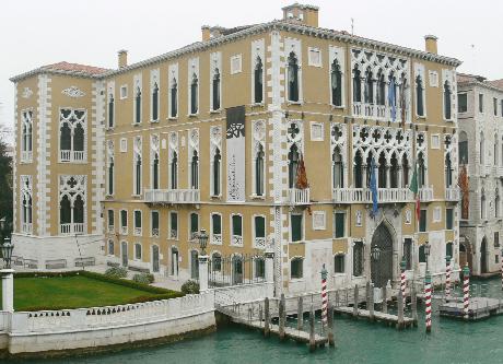
The conference “Neutrino Telescopes” has arrived at its XIII edition. It is a very nicely organized workshop, held in Venice every year towards the end of the winter or the start of the spring. For me it is especially pleasing to attend, since the venue, Palazzo Franchetti (see picture below) is located at a ten minute walk from my home: a nice change from my usual hour-long commute with Padova by train.
This year the conference will start on Tuesday, March 10th, and will last until Friday. I will be blogging from there, hopefully describing some new results heard in the several interesting talks that have been scheduled. Let me mention only a few of the talks, pasted from the program:
- D. Meloni (University of Roma Tre)
CP Violation in Neutrino Physics and New Physics - K. Hoffman (University of Maryland)
AMANDA and IceCube Results - S. Enomoto (Tohoku University)
Using Neutrinos to study the Earth - D.F. Cowen (Penn State University)
The Physics Potential of IceCube’s Deep Core Sub-Detector - S. Katsanevas (Université de Paris 7)
Toward a European Megaton Neutrino Observatory - E. Lisi (INFN, Bari)
Core-Collapse Supernovae: When Neutrinos get to know Each
Other - G. Altarelli (University of Roma Tre & CERN)
Recent Developments of Models of Neutrino Mixing - M. Mezzetto (INFN, Padova)
Next Challenge in Neutrino Physics: the θ13 Angle - M. Cirelli (IPhT-CEA, Saclay)
PAMELA, ATIC and Dark Matter
The conference will close with a round table: here are the participants:
Chair: N. Cabibbo (University of Roma “La Sapienza”)
B. Barish (CALTECH)
L. Maiani (CNR)
V.A. Matveev (INR of RAS, Moscow)
H. Minakata (Tokyo Metropolitan University)
P.J. Oddone (FNAL)
R. Petronzio (INFN, Roma)
C. Rubbia (CERN)
M. Spiro (CEA, Saclay)
A. Suzuki (KEK)
Needless to say, I look forward to a very interesting week!
Vernon Barger: perspectives on neutrino physics May 22, 2008
Posted by dorigo in cosmology, news, physics, science.Tags: cosmology, mixing angles, neutrino, neutrino experiments
comments closed
Yesterday morning Barger gave the first talk at PPC 2008, discussing the status and the perspectives of research in physics and cosmology with neutrinos. I offer my notes of his talk below.
Neutrinos mix among each other and have mass. There is a matrix connecting flavor and mass eigenstates, and the matrix is parametrized by three angles and a phase. To these can be addded two majorana phases for the neutrinoless double beta decay: 

What do we know about these parameters ? We are at the 10th year anniversary of the groundbreaking discovery of SuperKamiokande. This was then confirmed by other neutrino experiments: MACRO, K2K, MINOS. The new result by MINOS has a 6.5 sigma significance in the low energy region. This allows to measure the mass difference precisely. It is found that 

Solar neutrino oscillations are a mystery that existed for years. The flux of solar neutrinos was calculated by Bahcall, and there was a deficit. The deficit has an energy structure, as measured by the Gallium, Chlorine, and SuperK and SNO experiments by looking in neutrinos coming from different reactions -because of the different energy thresholds of the detectors: pp interactions, Beryllium 7, and Boron 8 neutrinos.
The interpretation of the data, which evolved over time, is now that the solar mixing angle is quite large, and what happens is that the high energy neutrinos sent here are created in the center of the sun, but they make a transition in matter, an adiabatic transition to a state 
There is a new result from Borexino, they measured neutrinos from the Beryllium line, and they reported a result consistent with others. Borexino is going to measure with 2% accuracy the deficit, and if KamLand has enough purity they can also go down to about 5% accuracy.
Kamland data provides a beautiful confirmation of the solution of the solar neutrino problem: solar parameters are measured precisely. 


There is one remaining angle to determine, 
What do we expect theoretically on
There is a model called tri-bimaximal mixing: a composition analogous to the quark model basis of neutral pions, eta and eta’ mesons. An intriguing matrix: it could be a new symmetry of nature, possibly softly broken with a slightly non-zero value of the angle 
So, we need to find what
Neutrinoless double-beta decay can tell us if the neutrinos are Majorana particles. In the inverted hierarchy, you measure the average mass versus the sum. There is a lot of experimental activity going on here.
Cosmic microwave has put a limit on sum of masses at 0.6 eV. By doing 21cm tomography one can measure neutrino masses with precision of 0.007 eV. If this is realizable, it could individually measure the masses of these fascinating particles.
Barger then mentioned the idea of mapping the universe with neutrinos: the idea is that active galactic nuclei (AGN) produce hadronic interactions with pions decaying to neutrinos, and there is a whole range of experiments looking at this. You could study the neutrinos coming from AGN and their flavor composition.
Another late-breaking development is that Auger has shown a correlation of ultra high-energy cosmic rays with AGNs in the sky: the cosmic rays seem to arrive directly from the nuclei of active galaxies. Auger found a higher correlation with sources at 100 Mpc, but falling off at higher distances. Cosmic rays are already probing the AGN, and this is very good news for neutrino experiments.
Then he discussed neutrinos from the sun: annihilation of weakly interacting massive particles (WIMPS), dark matter candidates, can give neutrinos from WW, ZZ, ttbar production. The idea is that the sun captured these particles gravitationally during its history, and the particles annihilate in the center of the sun, letting neutrinos escape with high energy. The ICECUBE discovery potential is high if the spin-dependent cross section for WIMP interaction in the sun is sufficiently high.
In conclusion, we have a rich panorama of experiments that all make use of neutrinos as probes of exotic phenomena as well as processes which we have to measure better to gain understanding of fundamental physics as well as gather information about the universe.
Denny Marfatia’s talk on Neutrinos and Dark Energy May 22, 2008
Posted by dorigo in astronomy, cosmology, news, physics, science.Tags: dark energy, fine structure constant, neutrino, oklo, PPC2008
comments closed
Denny spoke yesterday afternoon at PPC 2008. Below I summarize as well as I can those parts of his talk that were below a certain crypticity threshold (above which I cannot even take meaningful notes, it appears).
He started with a well-prepared joke: “Since at this conference the tendency is to ask questions early, Any questions ?“. This caused the hilarity of the audience, but indeed, as I noted in another post, the setting is relaxed and informal, and the audience interrupts loosely the speaker. Nobody seemed to complain so far…
Denny started by stating some observational facts: the dark energy (DE) density is 


But he noted that there is more than just one coincidence problem. In fact DE density and other densities have ratios which are small values. Within a factor of 10 the components are equal.
Why not consider these coincidences to have some fundamental origin ? Perhaps neutrino and DE densities are related. It is easy to play with this hypothesis with neutrinos because we understand them the least!
We can have the neutrino mass made a variable quantity. Imagine a fluid, the scalar, a quintessence scalar, and the potential is 
So one makes a decreasing neutrino mass at the minimum of the potential, with a varying potential. Some consequences of this model are given by the expression 
Neutrino masses can be made to vary with their number density: if w is close to -1, the effective potential has to scale with the neutrino contribution. Neutrinos are then most massive in empty space, and they are lighter when they cluster.
This could create an intriguing conflict between cosmological and terrestrial probes of neutrino mass. The neutrino masses vary with matter density if the scalar induces couplings to matter. There should be new matter effects in neutrino oscillations. One could also see temporal variations in the fine structure constant.
If neutrinos are light, DE becomes a cosmological constant, w = -1, and we cannot distinguish it from other models. Also, light neutrinos do not cluster, so the local neutrino mass will be the same as the background value; and high redshift data and tritium beta decay will be consistent because neither will show evidence for neutrino mass.
So one can look at the evidence for variations in time of the fine structure constant. The status of measurements of transition frequencies in atomic clocks give the limit 
The abundance ratio of Sm 149 to Sm147 at the natural reactor in Oklo shows no variation in the last 1.7 billion years, with a limit 
Resonant energy for neutron capture.
Meteoritic data (at a redshift z<0.5) constrain the beta decay rate of Rhenium 187 back to the time of solar system formation (4.6 Gy), 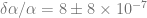
Going back to 

Then, there is a measurement of CMB (at z=1100) which determines 
Also primordial abundances from Big-bang nucleosynthesis (at z=10 billion) allow one to find
One can therefore hypothesize a phase transition in 
The first assumption is the following: M has a unique stationary point. Additional stationary points are possible, but for nonrelativistic neutrinos with subcritical neutrino density, only one minimum, fixed, and no evolution.
For non-relativistic neutrinos, with supercritical density, there is a window of instability.
You expect neutrinos at the critical density at some redshift. The instability can be avoided if the growth-slowing effects provided by cold dark matter dominate over the acceleron-neutrino coupling. Requiring no variation of 
