Guess the function: results January 21, 2009
Posted by dorigo in physics, science.Tags: bremsstrahlung, CMS, LHC, PDF, QCD, QED, Z boson
comments closed
Thanks to the many offers for help received a few days ago, when I asked for hints on possible functional forms to interpolate a histogram I was finding hard to fit, I have successfully solved the problem, and can now release the results of my study.
The issue is the following one: at the LHC, Z bosons are produced by electroweak interactions, through quark-antiquark annihilation. The colliding quarks have a variable energy, determined by probability density functions (PDF) which determine how much of the proton’s energy they carry; and the Z boson has a resonance shape which has a sizable width: 2.5 GeV, for a 91 GeV mass. The varying energy of the center of mass, determined by the random value of quark energies due to the PDF, “samples” the resonance curve, creating a distortion in the mass distribution of the produced Z bosons.
The above is not the end of the story, but just the beginning: in fact, there are electromagnetic corrections (QED) due to the radiation of photons, both “internally” and by the two muons into which the Z decays (I am focusing on that final state of Z production: a pair of high-momentum muons from 
Now, let us treat all of that as a black box: we only care to describe the mass distribution of muon pairs from Z production at the LHC, and we have a pretty good simulation program, Horace (developed by four physicists in Pavia University: C.M. Carloni Calame, G. Montagna, O. Nicrosini and A. Vicini), which handles the effects discussed above. My problem is to describe with a simple function the produced Z boson lineshape (the mass distribution) in different bins of Z rapidity. Rapidity is a quantity connected to the momentum of the particle along the beam direction: since the colliding quarks have variable energies, the Z may have a high boost along that direction. And crucially, depending on Z rapidity, the lineshape varies.
In the post I published here a few days ago I presented the residual of lineshape fits which used the original resonance form, neglecting all PDF and QED effects. By fitting those residuals with a proper parametrized function, I was trying to arrive at a better parametrization of the full lineshape.
After many attempts, I can now release the results. The template for residuals is shown below, interpolated with the function I obtained from an advice by Lubos Motl:

 After multiplying that function by the original Breit-Wigner resonance function, I could fit the 24 lineshapes extracted from a binning in rapidity. This produced additional residuals, which are of course much smaller than the first-order ones above, and have a sort of parabolic shape this time. A couple of them are shown on the right.
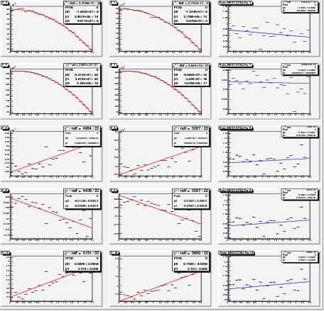
I then interpolated those residuals with parabolas, and extracted their fit parameters. Then, I could parametrize the parameters, as the graph below shows: the three degrees of freedom have roughly linear variations with Z rapidity. The graphs show the five parameter dependences on Z rapidity (left column) for lineshapes extracted with the CTEQ set of parton PDF; for MRST set (center column); and the ratio of the two parametrization (right column), which is not too different from 1.0.
Finally, the 24 fits which use the 

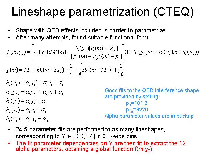
The function used is detailed in the slide below:
I am rather satisfied by the result, because the residuals of these final fits are really small, as shown on the right: they are certainly smaller than the uncertainties due to PDF and QED effects. The 

Some posts you might have missed in 2008 – part II January 6, 2009
Posted by dorigo in physics, science.Tags: anomalous muons, CDF, D0, Higgs boson, LHC, Lubos Motl, new physics, PDF, QCD, Tevatron, top mass, top quark, Z boson
comments closed
Here is the second part of the list of useful physics posts I published on this site in 2008. As noted yesterday when I published the list for the first six months of 2008, this list does not include guest posts nor conference reports, which may be valuable but belong to a different place (and are linked from permanent pages above). In reverse chronological order:
December 29: a report on the first measurement of exclusive production of charmonium states in hadron-hadron collisions, by CDF.
December 19: a detailed description of the effects of parton distribution functions on the production of Z bosons at the LHC, and how these effects determine the observed mass of the produced Z bosons. On the same topic, there is a maybe simpler post from November 25th.
December 8: description of a new technique to measure the top quark mass in dileptonic decays by CDF.
November 28: a report on the measurement of extremely rare decays of B hadrons, and their implications.
November 19, November 20, November 20 again , November 21, and November 21 again: a five-post saga on the disagreement between Lubos Motl and yours truly on a detail on the multi-muon analysis by CDF, which becomes a endless diatriba since Lubos won’t listen to my attempts at making his brain work, and insists on his mistake. This leads to a back-and-forth between our blogs and a surprising happy ending when Motl finally apologizes for his mistake. Stuff for expert lubologists, but I could not help adding the above links to this summary. Beware, most of the fun is in the comments threads!
November 8, November 8 again, and November 12: a three-part discussion of the details in the surprising new measurement of anomalous multi-muon production published by CDF (whose summary is here). Warning: I intend to continue this series as I find the time, to complete the detailed description of this potentially groundbreaking study.
October 24: the analysis by which D0 extracts evidence for diboson production using the dilepton plus dijet final state, a difficult, background-ridden signature. The same search, performed by CDF, is reported in detail in a post published on October 13.
September 23: a description of an automated global search for new physics in CDF data, and its intriguing results.
September 19: the discovery of the 
August 27: a report on the D0 measurement of the polarization of Upsilon mesons -states made up by a 
August 21: a detailed discussion of the ingredients necessary to measure with the utmost precision the mass of the W boson at the Tevatron.
August 8: the new CDF measurement of the lifetime of the 
August 7: a discussion of the new cross-section limits on Higgs boson production, and the first exclusion of the 170 GeV mass, by the two Tevatron experiments.
July 18: a search for narrow resonances decaying to muon pairs in CDF data excludes the tentative signal seen by CDF in Run I.
July 10: An important measurement by CDF on the correlated production of pairs of b-quark jets. This measurement is a cornerstone of the observation of anomalous multi-muon events that CDF published at the end of October 2008 (see above).
July 8: a report of a new technique to measure the top quark mass which is very important for the LHC, and the results obtained on CDF data. For a similar technique of relevance to LHC, also check this other CDF measurement.
More on the Z lineshape at LHC December 19, 2008
Posted by dorigo in personal, physics, science.Tags: CMS, momentum scale, PDF, Z boson
comments closed
Yesterday I posted a nice-looking graph without abounding in explanations on how I determined it. Let me fill that gap here today.
A short introduction
Z bosons will be produced copiously at the LHC in proton-proton collisions. What happens is that a quark from one proton hits an antiquark of the same flavour in the other proton, and the pair annihilates, producing the Z. This is a weak interaction: a relatively rare process, because weak interactions are much less frequent than strong interactions. Quarks carry colour charge as well as weak hypercharge, and most of the times when they hit each other what “reacts” is their colour, not their hypercharge. Similarly, when you meet John at the coffee machine you discuss football more often than chinese checkers: in particle physics terms, that is because your football coupling with John is stronger than your chinese-checkers coupling.
Result now, explanation later December 18, 2008
Posted by dorigo in personal, physics, science.Tags: CMS, momentum scale, PDF, Z boson
comments closed
Tonight I feel accomplished, since I have completed a crucial update of the cornerstone of the algorithm which provides the calibration of the CMS momentum scale. I have no time to discuss the details tonight, but I will share with you the final result of a complicated multi-part calculation (at least, for my mediocre standards): the probability distribution function of measuring the Z boson mass at a certain value 


The above might -and should, if you are not a HEP physicist- sound rather meaningless, but the family of two-dimensional functions 

Still confused ? No worry. Today I will only show one sample result – the probability distribution as a function of 

In the three-dimensional graph above, one axis has the reconstructed mass of muon pairs
The Z mass at a hadron collider November 25, 2008
Posted by dorigo in personal, physics, science.Tags: CMS, PDF, QCD, Z boson
comments closed
The Z boson mass has been measured with exquisite precision in the nineties by the LEP experiments ALEPH, OPAL, DELPHI and L3, and by the SLD experiment at SLAC: we know its value to better than a few MeV precision. The PDG gives 
For an experimental physicist, however, the knowledge of the Z mass is more a tool for calibration purposes than a key to theoretical investigations. Indeed, as I have discussed elsewhere recently, I am working at the calibration of the CMS tracker using the decays of Z bosons, as well as of lower-mass resonances. We take 
In CMS we will quickly collect large numbers of Z bosons, so statistics is not an issue: we will be able to study the calibration of tracks very effectively with those events. However, when statistics is large, experimentalists start worrying about systematic uncertainties. Indeed, there are several effects that cause a difference between the mass value we reconstruct with muon tracks and the true value of the Z boson mass -the one so well determined which sits in the PDG.
I decided to study one of those effects today: the mass shift due to parton distribution functions (PDF). When you collide protons against other protons, what creates a Z boson is the hard interaction between a quark and an antiquark. These constituents of the projectiles carry a fraction of the total proton momentum, but this fraction -called parton distribution function– is unknown on an event-by event basis. By studying proton collisions in different conditions and environments for a long time, we have been able to extract functions 
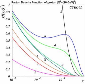 Now, things are complicated, because each different quark q (u,d,s,c,b) has its own different parton distribution function. The proton contains two valence up-quarks and one valence down-quark: it has a (uud) composition. Those quarks carry a good part of the proton’s momentum, but a large share is due to the rest of partons the proton is made of: sea quark-antiquark pairs, and gluons. Protons do carry antiquarks of all kinds -five in total-, as well as gluons, and these, too, get their own distribution function. A plot of the parton distribution functions of the proton (with a logarithmic x-axis to enhance the low-x behavior) is shown on the right. Note the bumps of u- and d- quark distributions, in blue and green, respectively: those bumps are due to the valence quark contributions.
In reality, things are even more complicated than what I discussed above: you do not simply get away with one function per each of the 11 partons I mentioned thsi far, because these functions have a value which depends on the energy at which you probe the proton, 


The reason for the weird behavior of parton distribution functions -their evolution with 
You have every reason to be confused now: I was talking about calibrating the CMS tracker using muons, and now we are deep into Quantum ChromoDynamics. What gives ? Well: Z bosons are created by quark-antiquark annihilations, and those are found inside the colliding protons with probabilities which depend on their momentum fraction x, and on the total collision energy Q. Since the PDF of quarks and antiquarks peak at very small values of x, the probability of a collision yielding a Z boson -which has a respectable mass of 91 GeV- is small. If the Z was lighter, more of them would be produced. Now, the Z boson is a resonance, and like every resonance, it has a finite width. What that means is that not all Z bosons have exactly the same mass: while the peak is at 91.186 GeV, the width is 2.5 GeV, which means that it is not infrequent for a Z boson to have a mass of 89, or 92 GeV, rather than the average value. This is described by the Z lineshape, a function called Breit-Wigner:
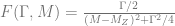
The function is shown below.
As you can see, there is a non-negligible probability that a Z boson has a mass quite different -even a few GeV off- from 91.19 GeV. Now, since Z bosons can be created at masses lower than 
The distorsion is very small, but it is very important to take it in account when one wants to use measured Z masses to precisely calibrate the track momentum measurement. To size up the effect of the PDF on the Z lineshape, one can compute an integral of the Breit-Wigner weighted with the PDF 
A Z can be produced by the following quark-antiquark interactions:
: this can originate from a valence u-quark and a sea anti-u-quark, as well as from a sea u-quark and a sea anti-u-quark. The probability that this quark pair creates a Z depends on the coupling of u-quarks to the Z boson, and this probability is a function of some coefficient predicted by electroweak theory. It is proportional to 0.11784.
: same as above, but the coupling is proportional to 0.15188.
: these can only occur through sea-sea interactions. The coefficient is the same as for d-quarks.
: these are due to the small charm component of the proton sea. They get the 0.11784 coefficient as u-quarks too.
: these are basically zero.
: gluon-gluon collisions cannot produce a Z boson, because they are vector particles as the Z (spin 1), and a vector-vector-vector vertex is zero by construction. Note that the same does not hold for the Higgs boson, which is a scalar (spin 0) particle: a vector-vector-scalar vertex is possible, and in fact it is the largest contribution to H production at the LHC.
 Putting everything together, one may compute the shift in the lineshape of the Z, and plot it directly (right, on a logarithmic scale to show the effect on the tails), or as a function of the rapidity of the Z boson, a quantity labeled by the letter Y (the dependence is shown in the last graph of this post, below). Rapidity is a measure of how fast is the Z boson moving in the detector reference frame: when one of the partons has a much larger momentum fraction than the one it is colliding against, the produced Z boson has a large momentum in the direction of the more energetic parton.
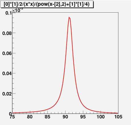
The rapidity distribution of Z bosons is shown in the graph below, separately for Zbosons produced by valence-sea collisions (in red) and by sea-sea collisions (in blue).
A rapidity Y=0 means that the Z was produced at rest in the detector, +5 is a fast-forward-moving Z, and -5 is a Z moving in the opposite direction with as much speed. As you can see, the valence-sea interactions are the most asymmetric ones, predominantly producing a forward-moving Z boson.
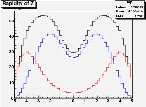
On the right here I also plot with the same color-coding the x distribution of quarks taking part in the Z creation. The red distribution has both a very small-x and a very large-x component, highlighting the asymmetric production.
Despite being in black and white, the most interesting plot is however the following one. It shows the average mass of the Z bosons (on the vertical scale, in GeV) as a function of the Z rapidity. The downward shift from 91.186 GeV is relevant -about 0.25 GeV overall- but it increases at large values of rapidity, when one of the two partons has a very small value of x, so that the collision “samples” a rapidly varying PDF for that parton.
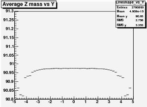 The plot on the left here is what is needed as an input for our calibration program: we will have to study how this dependence affects our determination of the momentum scale. A lot of work ahead, but a very enlightening one!
