Some recent posts you might want to read March 6, 2010
Posted by dorigo in Blogroll, internet, news, physics, science.Tags: B decays, CDF, CMS, Higgs boson, particle physics, quark, top quark, W boson, weak interactions
comments closed
As the less distracted among you know, I have moved my blogging activities to scientific blogging last April. I wish to report here a list of interesting posts I have produced there in the course of the last few months (precisely, since the start of 2010). They are given in reverse chronological order and with zero commentary – come see if you are curious.
- Understanding muon decay
- CDF on Higgs decays to diphotons
- Bose-Einstein interferences: the collider view
- Are quarks and leptons elementary or composite?
- Constraints on the Higgs mass from the muon anomaly
- Tevatron Higgs searches: past and future
- Exotic hadrons: there is the rub
- The fascinating search for rare W decays
- Three papers on the muon anomaly
- Particle physics in 2020
- Triggering: the subtle art of being picky
- New rare B decays nailed by CDF: a door to new physics?
- The approved CMS Phi signal with 900 GeV data
- Three top quarks: a door to new physics ?
- Luminosity, Michel Parameter, Phase space: what a lousy title for a great post
Things I should have blogged on last week April 13, 2009
Posted by dorigo in cosmology, news, physics, science.Tags: anomalous muons, CDF, dark matter, DZERO, Higgs boson, neutrino
comments closed
It rarely happens that four days pass without a new post on this site, but it is never because of the lack of things to report on: the world of experimental particle physics is wonderfully active and always entertaining. Usually hiatuses are due to a bout of laziness on my part. In this case, I can blame Vodafone, the provider of the wireless internet service I use when I am on vacation. From Padola (the place in the eastern italian Alps where I spent the last few days) the service is horrible, and I sometimes lack the patience to find the moment of outburst when bytes flow freely.
Things I would have wanted to blog on during these days include:
- The document describing the DZERO search of a CDF-like anomalous muon signal is finally public, about two weeks after the talk which announced the results at Moriond. Having had in my hands a unauthorized draft, I have a chance of comparing the polished with the unpolished version… Should be fun, but unfortunately unbloggable, since I owe some respect to my colleagues in DZERO. Still, the many issues I raised after the Moriond seminar should be discussed in light of an official document.
- DZERO also produced a very interesting search for
production. This is the associated production of a Higgs boson and a pair of top quarks, a process whose rate is made significant by the large coupling of top quarks and Higgs bosons, by virtue of the large top quark mass. By searching for a top-antitop signature and the associated Higgs boson decay to a pair of b-quark jets, one can investigate the existence of Higgs bosons in the mass range where the
decay is most frequent -i.e., the region where all indirect evidence puts it. However, tth production is invisible at the Tevatron, and very hard at the LHC, so the DZERO search is really just a check that there is nothing sticking out which we have missed by just forgetting to look there. In any case, the signature is extremely rich and interesting to study (I had a PhD doing this for CMS a couple of years ago), thus my interest.
- I am still sitting on my notes for Day 4 of the NEUTEL2009 conference in Venice, which included a few interesting talks on gravitational waves, CMB anisotropies, the PAMELA results, and a talk by Marco Cirelli on dark matter searches. With some effort, I should be able to organize these notes in a post in a few days.
- And new beautiful physics results are coming out of CDF. I cannot anticipate much, but I assure you there will be much to read about in the forthcoming weeks!
Just a link April 5, 2009
Posted by dorigo in Blogroll, news, physics, science.Tags: Higgs boson, science reporting, Tevatron
comments closed
I read with amusement (and some effort) a spanish account by Francis (th)E mule of Michael Dittmar’s controversial seminar of last March 19th. I paste the link here for several reasons: since I believe it might be of interest to some of you, to have a place to store it, and because I am not insensitive to flattery:
“Entre el público se encontraba Tomasso Dorigo […] (r)esponsable del mejor blog sobre física de partículas elementales del mundo”
Muchas gracias, Francis -but please note: my name spells with two m’s and one s!
Latest global fits to SM observables: the situation in March 2009 March 25, 2009
Posted by dorigo in news, physics, science.Tags: CDF, DZERO, electroweak fits, Gfitter, Higgs boson, LEP, SLD, standard model, Tevatron, top quark, W boson
comments closed
A recent discussion in this blog between well-known theorists and phenomenologists, centered on the real meaning of the experimental measurements of top quark and W boson masses, Higgs boson cross-section limits, and other SM observables, convinces me that some clarification is needed.
The work has been done for us: there are groups that do exactly that, i.e. updating their global fits to express the internal consistency of all those measurements, and the implications for the search of the Higgs boson. So let me go through the most important graphs below, after mentioning that most of the material comes from the LEP electroweak working group web site.
First of all, what goes in the soup ? Many things, but most notably, the LEP I/SLD measurements at the Z pole, the top quark mass measurements by CDF and DZERO, and the W mass measurements by CDF, DZERO, and LEP II. Let us give a look at the mass measurements, which have recently been updated.
For the top mass, the situation is the one pictured in the graph shown below. As you can clearly see, the CDF and DZERO measurements have reached a combined precision of 0.75% on this quantity.
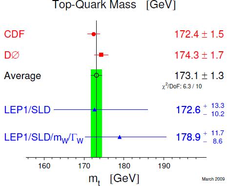
The world average is now at 


As far as global fits are concerned, there is one additional point to make for the top quark: knowing the top mass any better than this has become, by now, useless. You can see it by comparing the constraints on 
Then, let us look at the W mass determinations. Note, the graph below shows the situation BEFORE the latest DZERO result;, obtained with 1/fb of data, and which finds 
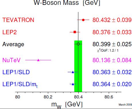
Here the situation is different: a better measurement would still increase the precision of our comparisons with indirect information from electroweak measurements at the Z. This is apparent by observing that the blue bars have width still smaller than the world average of direct measurements (again in green). Narrow the green band, and you can still collect interesting information on its consistency with the blue points.
Finally, let us look at the global fit: the electroweak working group at LEP displays in the by now famous “blue band plot”, shown below for March 2009 conferences. It shows the constraints on the Higgs boson mass coming from all experimental inputs combined, assuming that the Standard Model holds.
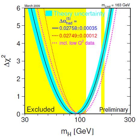
I will not discuss this graph in details, since I have done it repeatedly in the past. I will just mention that the yellow regions have been excluded by direct searches of the Higgs boson at LEP II (on the left, the wide yellow area) and the Tevatron ( the narrow strip on the right). From the plot you should just gather that a light Higgs mass is preferred (the central value being 90 GeV, with +36 and -27 GeV one-sigma error bars). Also, a 95% confidence-level exclusion of masses above 163 GeV is implied by the variation of the global fit 
I have started to be a bit bored by this plot, because it does not do the best job for me. For one thing, the LEP II limit and the Tevatron limit on the Higgs mass are treated as if they were equivalent in their strength, something which could not be possibly farther from the truth. The truth is, the LEP II limit is a very strong one -the probability that the Higgs has a mass below 112 GeV, say, is one in a billion or so-, while the limit obtained recently by the Tevatron is just an “indication”, because the excluded region (160 to 170 GeV) is not excluded strongly: there still is a one-in-twenty chance or so that the real Higgs boson mass indeed lies there.
Another thing I do not particularly like in the graph is that it attempts to pack too much information: variations of 

In this plot, the direct search results are introduced with their actual measured probability of exclusion as a function of Higgs mass, and not just in a digital manner, yes/no, as the yellow regions in the blue band plot. And in fact, you can see that the LEP II limit is a brick wall, while the Tevatron exclusion acts like a smooth increase in the global
From the black curve in the graph you can get a lot of information. For instance, the most likely values, those that globally have a 1-sigma probability of being one day proven correct, are masses contained in the interval 114-132 GeV. At two-sigma, the Higgs mass is instead within the interval 114-152 GeV, and at three sigma, it extends into the Tevatron-excluded band a little, 114-163 GeV, with a second region allowed between 181 and 224 GeV.
In conclusion, I would like you to take away the following few points:
- Future indirect constraints on the Higgs boson mass will only come from increased precision measurements of the W boson mass, while the top quark has exhausted its discrimination power;
- Global SM fits show an overall very good consistency: there does not seem to be much tension between fits and experimental constraints;
- The Higgs boson is most likely in the 114-132 GeV range (1-sigma bounds from global fits).
Zooming in on the Higgs March 24, 2009
Posted by dorigo in news, physics, science.Tags: CDF, DZERO, Higgs boson, LEP, MSSM, standard model, supersymmetry, Tevatron, top quark, W boson
comments closed
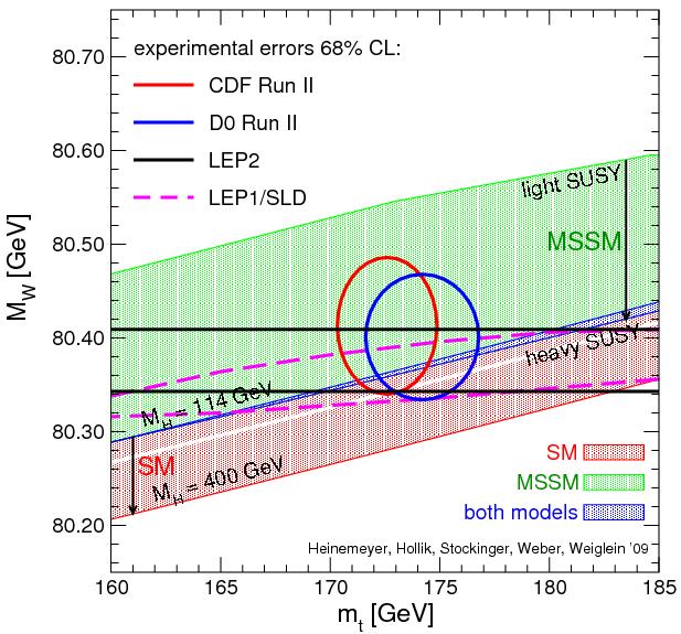 Yesterday Sven Heinemeyer kindly provided me with an updated version of a plot which best describes the experimental constraints on the Higgs boson mass, coming from electroweak observables measured at LEP and SLD, and from the most recent measurements of W boson and top quark masses. It is shown on the right (click to get the full-sized version).
The graph is a quite busy one, but I will try below to explain everything one bit at a time, hoping I keep things simple enough that a non-physicist can understand it.
The axes show suitable ranges of values of the top quark mass (varying on the horizontal axis) and of the W boson masses (on the vertical axis). The value of these quantities is functionally dependent (because of quantum effects connected to the propagation of the particles and their interaction with the Higgs field) on the Higgs boson mass.
The dependence, however, is really “soft”: if you were to double the Higgs mass by a factor of two from its true value, the effect on top and W masses would be only of the order of 1% or less. Because of that, only recently have the determinations of top quark and W boson masses started to provide meaningful inputs for a guess of the mass of the Higgs.
Top mass and W mass measurements are plotted in the graphs in the form of ellipses encompassing the most likely values: their size is such that the true masses should lie within their boundaries, 68% of the time. The red ellipse shows CDF results, and the blue one shows DZERO results.
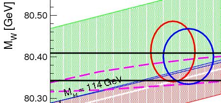 There is a third measurement of the W mass shown in the plot: it is displayed as a horizontal band limited by two black lines, and it comes from the LEP II measurements. The band also encompasses the 68% most likely W masses, as ellipses do.
In addition to W and top masses, other experimental results constrain the mass of top, W, and Higgs boson. The most stringent of these results are those coming from the LEP experiment at CERN, from detailed analysis of electroweak interactions studied in the production of Z bosons. A wide band crossing the graph from left to right, with a small tilt, encompasses the most likely region for top and W masses.
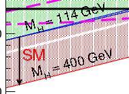 So far we have described measurements. Then, there are two different physical models one should consider in order to link those measurements to the Higgs mass. The first one is the Standard Model: it dictates precisely the inter-dependence of all the parameters mentioned above. Because of the precise SM predictions, for any choice of the Higgs boson mass one can draw a curve in the top mass versus W mass plane. However, in the graph a full band is hatched instead. This correspond to allowing the Higgs boson mass to vary from a minimum of 114 GeV to 400 GeV. 114 GeV is the lower limit on the Higgs boson mass found by the LEP II experiments in their direct searches, using electron-positron collisions; while 400 GeV is just a reference value.
The boundaries of the red region show the functional dependence of Higgs mass on top and W masses: an increase of top mass, for fixed W mass, results in an increase of the Higgs mass, as is clear by starting from the 114 GeV upper boundary of the red region, since one then would move into the region, to higher Higgs masses. On the contrary, for a fixed top mass, an increase in W boson mass results in a decrease of the Higgs mass predicted by the Standard Model. Also note that the red region includes a narrow band which has been left white: it is the region corresponding to Higgs masses varying between 160 and 170 GeV, the masses that direct searches at the Tevatron have excluded at 95% confidence level.
 The second area, hatched in green, is not showing a single model predictions, but rather a range of values allowed by varying arbitrarily many of the parameters describing the supersymmetric extension of the SM called “MSSM”, its “minimal” extension. Even in the minimal extension there are about a hundred additional parameters introduced in the theory, and the values of a few of those modify the interconnection between top mass and W mass in a way that makes direct functional dependencies in the graph impossible to draw. Still, the hatched green region shows a “possible range of values” of the top quark and W boson masses. The arrow pointing down only describes what is expected for W and top masses if the mass of supersymmetric particles is increased from values barely above present exclusion limits to very high values.
So, to summarize, what to get from the plot ? I think the graph describes many things in one single package, and it is not easy to get the right message from it alone. Here is a short commentary, in bits.
- All experimental results are consistent with each other (but here, I should add, a result from NuTeV which finds indirectly the W mass from the measured ratio of neutral current and charged current neutrino interactions is not shown);
- Results point to a small patch of the plane, consistent with a light Higgs boson if the Standard Model holds
- The lower part of the MSSM allowed region is favored, pointing to heavy supersymmetric particles if that theory holds
- Among experimental determinations, the most constraining are those of the top mass; but once the top mass is known to within a few GeV, it is the W mass the one which tells us more about the unknown mass of the Higgs boson
- One point to note when comparing measurements from LEP II and the Tevatron experiments: when one draws a 2-D ellipse of 68% contour, this compares unfavourably to a band, which encompasses the same probability in a 1-D distribution. This is clear if one compares the actual measurements: CDF
(with 200/pb of data), DZERO
(with five times more statistics), LEP II
(average of four experiments). The ellipses look like they are half as precise as the black band, while they are actually only 30-40% worse. If the above is obscure to you, a simple graphical explanation is provided here.
- When averaged, CDF and DZERO will actually beat the LEP II precision measurement -and they are sitting on 25 times more data (CDF) or 5 times more (DZERO).
A seminar against the Tevatron! March 20, 2009
Posted by dorigo in news, physics, science.Tags: CDF, DZERO, Higgs boson, LHC, Tevatron
comments closed
I spent this week at CERN to attend the meetings of the CMS week – an event which takes place four times a year, when collaborators of the CMS experiment, coming from all parts of the world, get together at CERN to discuss detector commissioning, analysis plans, and recent results. It was a very busy and eventful week, and only now, sitting on a train that brings me back from Geneva to Venice, can I find the time to report with the due dedication on some things you might be interested to know about.
One thing to report on is certainly the seminar I eagerly attended on Thursday morning, by Michael Dittmar (ETH-Zurich). Dittmar is a CMS collaborator, and he talked at the CERN theory division on a tickling subject:”Why I never believed in the Tevatron Higgs sensitivity claims for Run 2ab”. The title did promise a controversial discussion, but I was really startled by its level, as much as by the defamation of which I felt personally to be a target. I will explain this below.
I have also to mention that by Thursday I had already attended to a reduced version of his talk, since he had given it on the previous day in another venue. Both I and John Conway had corrected him on a few plainly wrong statements back then, but I was puzzled to see he reiterated those false statements in the longer seminar! More on that below.
Dittmar’s obnoxious seminar
Dittmar started by saying he was infuriated by the recent BBC article where “a statement from the director of a famous laboratory” claimed that the Tevatron had 50% odds of finding a Higgs boson, in a certain mass range. This prompted him to prepare a seminar to express his scepticism. However, it turned out that his scepticism was not directed solely at the optimistic statement he had read, but at every single result on Higgs searches that CDF and DZERO had produced since Run I.
In order to discuss sensitivity and significances, the speaker made a un-illuminating digression on how counting experiments can or cannot obtain observation-level significances with their data depending on the level of background of their searches and the associated systematical uncertainties. His statements were very basic and totally uncontroversial on this issue, but he failed to focus on the fact that nowadays, nobody does counting experiments any more when searching for evidence of a specific model: our confidence in advanced analysis methods involving neural networks, shape analysis, and likelihood discriminants; the tuning of Monte Carlo simulations; and the accurate analytical calculations of high-order diagrams for Standard Model processes, have all grown tremendously with years of practice and studies, and these methods and tools overcome the problems of searches for small signals immersed in large backgrounds. One can be sceptical, but one cannot ignore the facts, as the speaker seemed inclined to.
Then Dittmar said that in order to judge the value of sensitivity claims for the future, one may turn to past studies and verify their agreement with the actual results. So he turned to the Tevatron Higgs Sensitivity studies of 2000 and 2003, two endeavours to which I had participated with enthusiasm.
He produced a plot showing the small signal of 
He commented that figure by saying half-mockingly that the data could have been used to exclude the standard model process of associated 
In fact, he went on to discuss the global expectation of the Tevatron on Higgs searches, a graph (see below) produced in 2000 after a big effort from several tens of people in CDF and DZERO.

He started by saying that the graph was confusing, and that it was not clear in the documentation how it had been produced, nor that it was the combination of CDF and DZERO sensitivity. This was very amusing, since sitting from the far back John Conway, a CDF colleague, shouted: “It says it in print on top of it: combined thresholds!”, then adding, with a pacate voice “…In case you’re wondering, I made that plot.” John had in fact been the leader of the Tevatron Higgs sensitivity study, not to mention the author of many of the most interesting searches for the higgs boson in CDF since then.
Dittmar continued his surreal talk with an overbid, by claiming that the plot had been produced “by assuming a 30% improvement in the mass resolution of pairs of b-jets, when nobody had not even the least idea on how such improvement could be achieved”.
I could not have put together a more personal, direct attack to years of my own work myself! It is no mystery that I worked on dijet resonances since 1992, but of course I am a rather unknown soldier in this big game; however, I felt the need to interrupt the speaker at this point -exactly as I had done at the shorter talk the day before.
I remarked that in 1998, one year before the Tevatron sensitivity study, I had produced a PhD thesis and public documents showing the observation of a signal of 


In the plots, you can see how the excess over background predictions moves to the right as more and more refined jet energy corrections are applied, starting from the result of generic jet energy corrections (top) to optimized corrections (bottom) until the signal becomes narrower and centered at the true value. The plots on the left show the data and the background prediction, those on the right show the difference, which is due to Z decays to b-quark jet pairs. Needless to say, the optimization is done on Monte Carlo Z events, and only then checked on the data.
So I said that Dittmar’s statement was utterly false: we had an idea of how to do it, we had proven we could do it, and besides, the plots showing what we had done had been indeed included in the Tevatron 2000 report. Had he overlooked them ?
Escalation!
Dittmar seemed unbothered by my remark, and he responded that that small signal had not been confirmed in Run II data. His statement constituted an even more direct attack to four more years of my research time, spent on that very topic. I kept my cool, because when your opponent offers you on a silver plate the chance to verbally sodomize him, you cannot be too angry with him.
I remarked that a signal had indeed been found in Run II, amounting to about 6000 events after all selection cuts; it confirmed the past results. Dittmar then said that “to the best of his knowledge” this had not been published, so it did not really count. I then explained it was a 2008 NIM publication, and would he please document himself before making such unsubstantiated allegations? He shrugged his shoulders, said he would look more carefully for the paper, and went back to his talk.
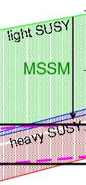
 His points about the Tevatron sensitivity studies were laid down: for a low-mass Higgs boson, the signal is just too small and backgrounds are too large, and the sensitivity of real searches is below expectations by a large factor. To stress this point, he produced a slide containing a plot he had taken from this blog! The plot (see on the left), which is my own concoction and not Tevatron-approved material, shows the ratio between observed limit to Higgs production and the expectations of the 2000 study. He pointed at the two points for 100-140 GeV Higgs boson masses, trying to prove his claim: The Tevatron is now doing three times worse than expected. He even uttered “It is time to confess: the sensitivity study was wrong by a large factor!”.
I could not help interrupting again: I had to stress that the plot was not approved material and was just a private interpretation of Tevatron results, but I did not deny its contents. The plot was indeed showing that low-mass searches were below par, but it was also showing that high-mass ones were amazingly in agreement with expectations worked at 10 years before. Then John Conway explained the low-mass discrepancy for the benefit of the audience, as he had done one day before for no apparent benefit of the speaker.
Conway explained that the study had been done under the hypothesis that an upgrade of our silicon detector would be financed by the DoE: it was in fact meant to prove the usefulness of funding an upgrade. A larger acceptance of inner silicon tracking boosts the sensitivity to identify b-quark jets from Higgs decays by a large factor, because any acceptance increase gets squared when computing the over-efficiency. So Dittmar could not really blame the Tevatron experiments for predicting something that would not materialize in a corresponding result, given that the DoE had denied the funding to build the upgraded detector!
I then felt compelled to add that by using my plot Dittmar was proving the opposite thesis of what he wanted to demonstrate: low-mass Tevatron searches were shown to underperform because of funding issues, rather than because of a wrong estimate of sensitivity; and high-mass searches, almost unhindered by the lack of an upgraded silicon, were in excellent agreement with expectations!
The speaker said that no, the high-mass searches were not in agreement, because their results could not be believed, and moved on to discuss those by taking real-data results by the Tevatron.
He said that the 
“Possible at the Tevatron ? I believe that the WW continuum background is much larger at a ppbar collider than at a pp collider, so my personal conclusion is that if the Tevatron people want to waste their time on it, good luck to them.”
Now, come on. I cannot imagine how a respectable particle physicist could drive himself into making such statements in front of a distinguished audience (which, have I mentioned it, included several theorists of the highest caliber, including none less than Edward Witten). Waste their time ? I felt I was wasting my time listening to him, but my determination of reporting his talk here kept me anchored to my chair, taking notes.
So this second part of the talk was not less unpleasant than the first part: Dittmar criticized the Tevatron high-mass Higgs results in the most incorrect, and scientifically dishonest, way that I could think of. Here is just a summary:
- He picked up a distribution of one particular sub-channel from one experiment, noting that it seemed to have the most signal-rich region showing a deficit of events. He then showed the global CDF+DZERO limit, which did not show a departure between expected and observed limit on Higgs cross section, and concluded that there was something fishy in the way the limit had been evaluated. But the limit is extracted from literally several dozens of those distributions -something he failed to mention despite having been warned of that very issue in advance.
- He picked up two neural-network output distributions for a search of Higgs at 160 and 165 GeV, and declared they could not be correct since they were very different in shape! John, from the back, replied “You have never worked with neural networks, have you ?” No, he had not. Had he, he would probably have understood that different mass points, optimized differently, can provide very different NN outputs.
- He showed another Neural Network output based on 3/fb of data, which had a pair of data points lying one standard deviation above the background predictions, and the corresponding plot for a search performed with improved statistics, which had instead a underfluctuation. He said he was puzzled by the effect. Again, some intervention from the audience was necessary, explaining that the methods are constantly reoptimized, and there is no wonder that adding more data can result in a different outcome. This produced a discussion when somebody from the audience tried to speculate that searches were maybe performed by looking at the data before choosing which method to use for a limit extraction! On the contrary of course, all Tevatron searches of the Higgs are blind analyses, where the optimization is performed on expected limits, using control samples, and Monte Carlo, and the data is only looked at afterwards.
- He showed that the Tevatron 2000 report had estimated a maximum Signal/Noise ratio for the H–>WW search of 0.34, and he picked up one random plot from the many searches of that channel by CDF and DZERO, showing that the signal to noise there was never larger than 0.15 or so. Explaining to him that the S/N of searches based on neural networks and combined discriminants is not a fixed value, and that many improvements have occurred in data analysis techniques in 10 years was useless.
Dittmar concluded his talk by saying that:
“Optimistic expectations might help to get funding! This is true, but it is also true that this approach eventually destroys some remaining confidence in science of the public.”.
His last slide even contained the sentence he had previously brought himself to uttering:
“It is the time to confess and admit that the sensitivity predictions were wrong”.
Finally, he encouraged LHC experiments to looking for the Higgs where the Tevatron had excluded it -between 160 and 170 GeV- because Tevatron results cannot be believed. I was disgusted: he most definitely places a strong claim on the prize of the most obnoxious talk of the year. Unfortunately for all, it was just as much an incorrect, scientifically dishonest, and dilettantesque lamentation, plus a defamation of a community of 1300 respected physicists.
In the end, I am really wondering what really moved Dittmar to such a disastrous performance. I think I know the answer, at least in part: he has been an advocate of the
Tevatron excludes chunk of Higgs masses! March 13, 2009
Posted by dorigo in news, physics, science.Tags: CDF, DZERO, Higgs boson, Tevatron
comments closed
This just in – the Fermilab site has the news on the new exclusion in a range of Higgs masses. At 95% C.L., the Higgs boson cannot have a mass in the 160-170 GeV range, as shown in the graph below. The new limit is shown by the orange band.

This is the first real exclusion range on the Higgs boson mass from CDF and DZERO. I will have more to say about this great new result during the weekend.
UPDATE: maybe the most interesting thing is not the limit shown above, but the information contained in the graph shown below. It shows how the combination of CDF and DZERO searches for the Higgs bosons end up agreeing with the background-only hypothesis (black hatched curve) or the background plus signal hypothesis (red curve), as a function of the unknown value of the Higgs boson mass. The full black line seems to favor the signal plus background hypothesis, although only marginally and at just the 1-sigma level, at around 130 GeV of mass:

However, they say that if you like sausages and if you follow laws, you should not ask how these things are made. The same goes with global limits, to some extent. In this case it is not a criticism of the limit by itself, but rather of the interpretation that one might be led to give to it. In fact, the width of the green band should put you en garde against wild speculations: It would be extremely suspicious if the black line did not venture outside of the green band somewhere, even in case the Higgs boson does not exist!
That is because the band shows the expected range of 1-sigma fluctuations -due to statistical effects, and not to systematic ones such as the real presence of a signal!- and since the black curve is extracted from the data by combining many datasets and each individual point of the line (in, say, 5-GeV intervals) has little correlation with the others, it is entirely appropriate for the curve to not be fully contained in the green area! So, the fact that the black curve overlaps with the signal plus background hypothesis at 130 GeV really -really!- means very, very little.
What does mean something is that the hatched black and red curves appear separated by about one-sigma (the width of the green band surrounding the background-only black hatched curve) over a wide range of Higgs masses. This says that the two Tevatron experiments have by now reached a sensitivity of about 1-sigma to the signal with the data they have analyzed so far. Beware: they are already sitting on about twice as much data (most analyses rely on about 2.5/fb of collisions, but the Tevatron has already delivered to the experiments over 5/fb). So they expect new results, significantly improved, by this summer.
It does seem that at last, the game of Higgs hunting is starting to get exciting again, after a hiatus of about 7 years following the tentative signal seen by the LEP II experiments!
Higgs decays to photon pairs! March 4, 2009
Posted by dorigo in news, physics, science.Tags: DZERO, Higgs boson, LHC, photons, standard model, Tevatron
comments closed
It was with great pleasure that I found yesterday, in the public page of the DZERO analyses, a report on their new search for Higgs boson decays to photon pairs. On that quite rare decay process -along with another not trivial decay, the 
My delight was increased when I saw that results of the DZERO search are based on a data sample corresponding to a whooping 4.2 inverse-femtobarns of integrated luminosity. This is the largest set of hadron-collider data ever used for an analysis. 4.2 inverse femtobarns correspond to about three-hundred trillion collisions, sorted out by DZERO. Of course, both DZERO and CDF have so far collected more than that statistics: almost five inverse femtobarns. However, it always takes some time before calibration, reconstruction, and production of the newest datasets is performed… DZERO is catching up nicely with the accumulated statistics, it appears.
The most interesting few tens of billions or so of those events have been fully reconstructed by the software algorithms, identifying charged tracks, jets, electrons, muons, and photons. Yes, photons: quanta of light, only very energetic ones: gamma rays.
When photons have an energy exceeding a GeV or so (i.e. one corresponding to a proton mass or above), they can be counted and measured individually by the electromagnetic calorimeter. One must look for very localized energy deposits which cannot be spatially correlated with a charged track: something hits the calorimeter after crossing the inner tracker, but no signal is found there, implying that the object was electrically neutral. The shape of the energy deposition then confirms that one is dealing with a single photon, and not -for instance- a neutron, or a pair of photons traveling close to each other. Let me expand on this for a moment.
Background sources of photon signals
In general, every proton-antiproton collision yield dozens, or even hundreds of energetic photons. This is not surprising, as there are multiple significant sources of GeV-energy gamma rays to consider.
 Electrons, as well as in principle any other electrically charged particle emitted in the collision, have the right to produce photons by the process called bremsstrahlung: by passing close to the electric field generated by a heavy nucleus, the particle emits electromagnetic radiation, thus losing a part of its energy. Note that this is a process which cannot happen in vacuum, since there are no target nuclei there to supply the electric field with which the charged particle interacts (one can have bremsstrahlung also in the presence of neutral particles, in principle, since what matters is the capability of the target to absorb a part of the colliding body’s momentum; but in that case, one needs a more complicated scattering process, so let us forget about it). For particles heavier than the electron, the process is suppressed up to the very highest energy (where particle masses are irrelevant with respect to their momenta), and is only worth mentioning for muons and pions in heavy materials.
- By far the most important process for photon creation at a collider is the decay of neutral hadrons. A high-energy collision at the Tevatron easily yields a dozen of neutral pions, and these particles decay more than 99% of the time into pairs of photons,
. Of course, these photons would only have an energy equal to half the neutral pion mass -0.07 GeV- if the neutral pions were at rest; it is only through the large momentum of the parent that the photons may be energetic enough to be detected in the calorimeter.
- A similar fate to that of neutral pions awaits other neutral hadrons heavier than the
: most notably the particle called eta, in the decay
. The eta has a mass four times larger than that of the neutral pion, and is less frequently produced.
- And other hadrons may produce photons in de-excitation processes, albeit not in pairs: excited hadrons often decay radiatively into their lower-mass brothers, and the radiated photon may display a significant energy, again critically depending on the parent’s speed in the laboratory.
All in all, that’s quite a handful of photons our detectors are showered with on an event-by-event basis! How the hell can DZERO sort out then, amidst over three hundred trillion collisions, the maybe five or ten which saw the decay of a Higgs to two photons ?
And the Higgs signal amounts to…
Five to ten events. Yes, we are talking of a tiny signal here. To eyeball how many standard model Higgs boson decays to photon pairs we may expect in a sample of 4.2 inverse femtobarns, we make some approximations. First of all, we take a 115 GeV Higgs for a reference: that is the Higgs mass where the analysis should be most sensitive, if we accept that the Higgs cannot be much lighter than that: for heavier higgses, their number will decrease, because the heavier a particle is, the less frequently it is produced.
The cross-section for the direct-production process 
The other input we need is the branching ratio of H decay to two photons. This is the fraction of disintegrations yielding the final state that DZERO has been looking for. It depends on the detailed properties of the Higgs particle, which likes to couple to particles depending on the mass of the latter. The larger a particle’s mass, the stronger its coupling to the Higgs, and the more frequent the H decay into a pair of those: the branching fraction depends on the squared mass of the particle, but since the sum of all branching ratios is one -if we say the Higgs decays, then there is a 100% chance of its decaying into something, no less and no more!- any branching fraction depends on ALL other particle masses!!!
 “Wait a minute,” I would like to hear you say now, “the photon is massless! How can the Higgs couple to it?!”. Right. H does not couple directly to photons, but it can nevertheless decay into them via a virtual loop of electrically charged particles. Just as happens when your US plug won’t fit into an european AC outlet! You do not despair, and insert an adaptor: something endowed with the right holes on one side and pins on the other. Much in the same way, a virtual loop of top quarks, for instance, will do a good job: the top has a large mass -so it couples aplenty to the Higgs- and it has an electric charge, so it is capable of emitting photons. The three dominant Feynman diagrams for the
So, how much is the branching ratio to two photons in the end ? It is a complicated calculus, but the result is roughly one thousandth. One in a thousand low-mass Higgses will disintegrate into energetic light: two angry gamma rays, each roughly carrying the energy of a 2 milligram mosquito launched at the whooping speed of four inches per second toward your buttocks.
Now we have all the ingredients for our computation of the number of signal events we may be looking at, amidst the trillions produced. The master formula is just

where 


With 

The DZERO analysis
I will not spend much of my and your time discussing the details of the DZERO analysis here, primarily because this post is already rather long, but also because the analysis is pretty straightforward to describe at an elementary level: one selects events with two photons of suitable energy, computes their combined invariant mass, and compares the expectation for Higgs decays -a roughly bell-shaped curve centered at the Higgs mass and with a width of ten GeV or so- with the expected backgrounds from all the processes capable of yielding pairs of energetic photons, plus all those yielding fake photons. [Yes, fake photons: of course the identification of gamma rays is not perfect -one may have not detected a charged track pointing at the calorimeter energy deposit, for instance.] Then, a fit of the mass distribution extracts an upper limit on the number of signal events that may be hiding there. From the upper limit on the signal size, an upper limit is obtained on the signal cross-section.
Ok, the above was a bit too quick. Let me be slightly more analytic. The data sample is collected by an online trigger requiring two isolated electromagnetic deposits in the calorimeter. Offline, the selection requires that both photon candidates have a transverse energy exceeding 25 GeV, and that they be isolated from other calorimetric activity -a requirement which removes fake photons due to hadronic jets.
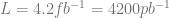
Further, there must be no charged tracks pointing close to the deposit, and a neural-network classifier is used to discriminate real photons from backgrounds using the shape of the energy deposition and other photon quality variables. The NN output is shown in the figure below: real photons (described by the red histogram) cluster on the right. A cut on the data (black points) of a NN output larger than 0.1 accepts almost all signal and removes 50% of the backgrounds (the hatched blue histogram). One important detail: the shape of the NN output for real high-energy photons is modeled by Monte Carlo simulations, but is found in good agreement with that of real photons in radiative Z boson decay processes, 
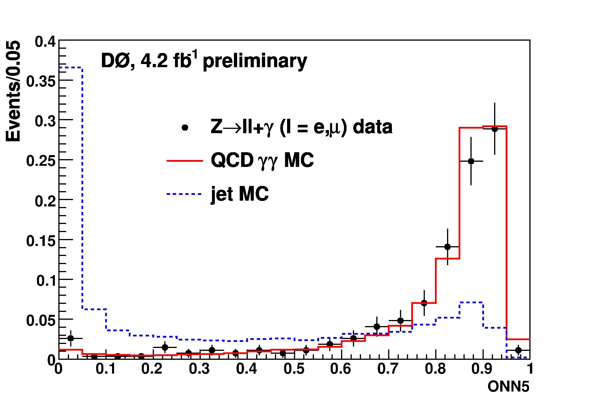
After the selection, surviving backgrounds are due to three main processes: real photon pairs produced by quark-antiquark interactions, compton-like gamma-jet events where the jet is mistaken for a photon, and Drell-Yan processes yielding two electrons, both of which are mistaken for photons. You can see the relative importance of the three sources in the graph below, which shows the diphoton invariant mass distribution for the data (black dots) compared to the sum of backgrounds. Real photons are in green, compton-like gamma-jet events are in blue, and the Drell-Yan contribution is in yellow.
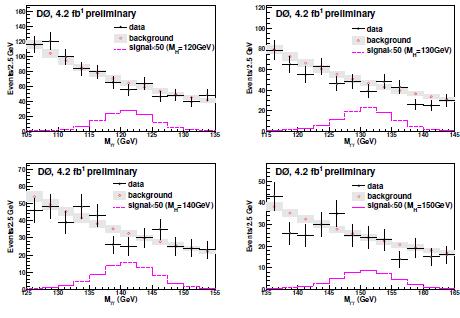
The mass distribution has a very smooth exponential shape, and to search for Higgs events DZERO fits the spectrum with an exponential, obliterating a signal window where Higgs decays may contribute. The fit is then extrapolated into the signal window, and a comparison with the data found there provides the means for a measurement; different signal windows are assumed to search for different Higgs masses. Below are shown four different hypotheses for the Higgs mass, ranging from 120 to 150 GeV in 10-GeV intervals. The expected signal distribution, shown in purple, is multiplied by a factor x50 in the plots, for display purposes.
From the fits, a 95% upper limit on the Higgs boson production cross section is extracted by standard procedures. As by now commonplace, the cross-section limit is displayed by dividing it by the expected standard model Higgs cross section, to show how far one is from excluding the SM-produced Higgs at any mass value. The graph is shown below: readers of this blog may by now recognize at first sight the green 1-sigma and yellow 2-sigma bands showing the expected range of limits that the search was predicted to set. The actual limit is shown in black.
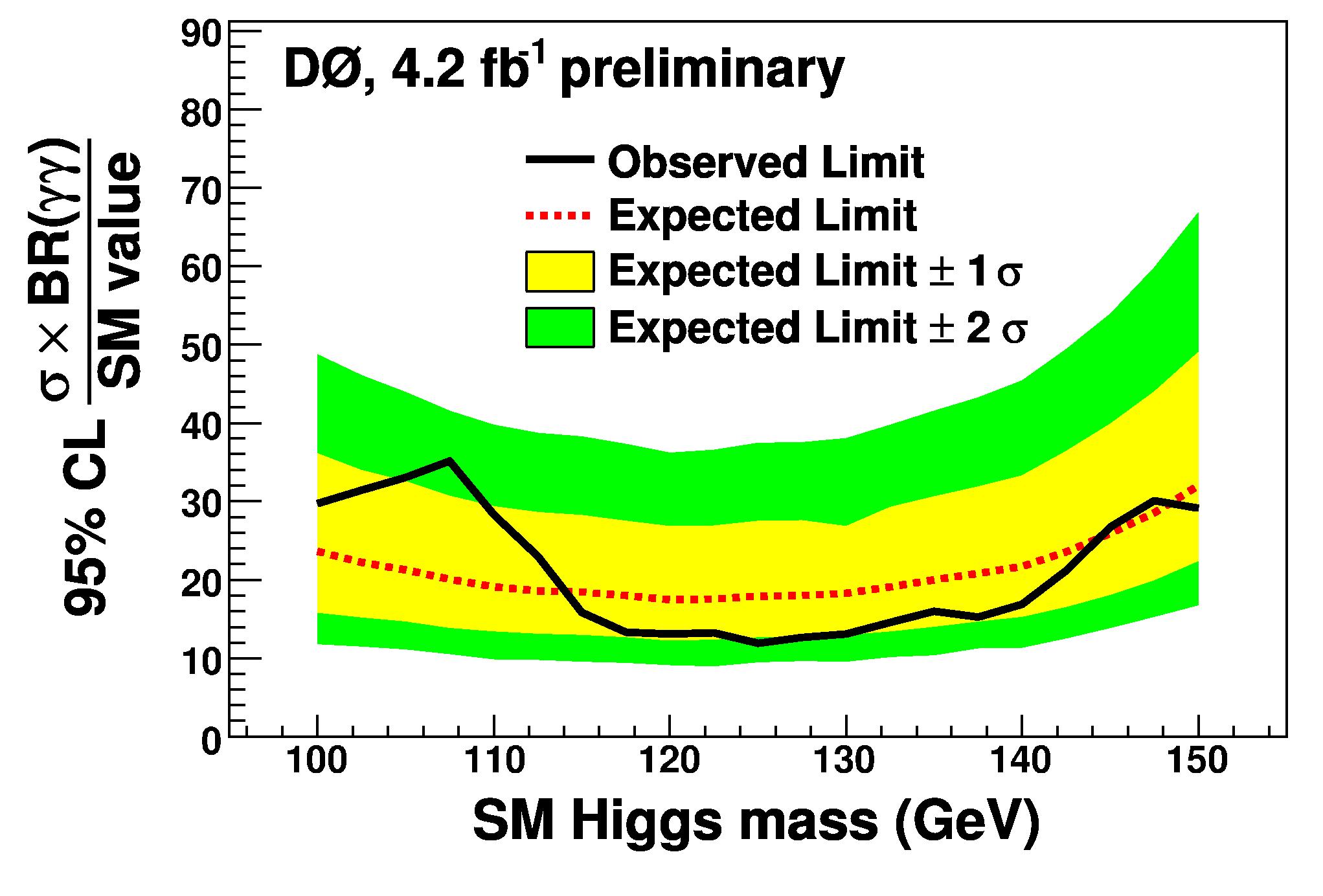
One notices that while this search is not sensitive to the Higgs boson yet, it is not so far from it any more! The LHC experiments will have a large advantage with respect to DZERO (and CDF) in this particular business, since there the Higgs production cross-section is significantly larger. Backgrounds are also larger, however, so a detailed understanding of the detectors will be required before such a search is carried out with success at the LHC. For the time being, I congratulate with my DZERO colleagues for pulling off this nice new result!
Notes on the new Higgs boson search by DZERO March 2, 2009
Posted by dorigo in news, physics, science.Tags: D0, Higgs boson, neural networks, standard model, Tevatron
comments closed
Three weeks ago the DZERO collaboration published new results of their low-mass Higgs boson search. This is about the production of Higgs bosons in association with a W boson, with the subsequent decay of the Higgs particle to a pair of b-quark jets, and the decay of the W to an electron-electron neutrino or muon- muon neutrino pair: in symbols, what I mean is 

In order to make this blog more accessible than it would otherwise be, I frequently write things inaccurately: precision is usually pedantic and distracting. But here I beg you to please note a detail I will not gloss over for once: to be accurate, one should write 
Two words on associated WH production and its merits
The associated production of the Higgs together with a W boson is the “golden” signature for low-mass Higgs hunters at the Tevatron collider. While producing the Higgs together with another heavy object is not effortless (you are required to produce the collision with more energetic quarks in the two colliding protons, and this makes the production less frequent), the W boson pays back with extra dividends by producing a very clean signature in its leptonic decay, and by allowing the event to be spotted easily by the online triggering system, and collected with high efficiency by the data acquisition.
If you compare the collection of WH events to the collection of directly produced Higgs bosons (

Higgs decays to b-quark pairs produced alone simply cannot be triggered in hadronic collisions, because they are immersed in a background which is six orders of magnitude higher in rate, namely the production 
Yes, life is tough for hadronic signatures at a hadron collider. Even finding the
The DZERO analysis
The new analysis by DZERO studies a total integrated luminosity of 2.7 inverse femtobarns. This corresponds to 150 trillion proton-antiproton collisions, but DZERO has netted almost twice as much data already by now, and it is only a matter of time before those too get included in this search: so one has to bear in mind that the statistical power of the data is soon going to increase by about 40%: the data increase corresponds to an increase in precision by the square root of two, or a factor of 1.41.
DZERO selects events which have an electron or a muon with high energy -the tag of a leptonic decay of the W boson-, missing transverse energy, and two or three hadronic jets. The presence of a energy imbalance in the plane transverse to the beam direction is a comparatively clean signature of the escape of the energetic neutrino produced together with the charged lepton by the W decay, and two jets are expected from the decay of the Higgs boson to a pair of b quarks. However, you might well ask, quid opus fuit tertium ?
No, I bet you would not ask it that way -for some reason, a reminescence of Latin sprung up in my mind. Quid opus fuit tertium – What is the matter with the third one ? The third jet is not specifically a signature of any one of the decay products of the WH pair we are after. However, if you remember what I mentioned above, we are searching for inclusive production of a WH pair: that means we accept the fact that the two projectiles also produced an additional energetic stream of hadrons in the final state. That possibility is by no means rare, and in fact it amounts to about 20% of the Higgs production events. By selecting events with two or three jets, DZERO increases its acceptance of signal events sizably.
A technique which has become commonplace in the hunt of elusive subnuclear particles is to slice and dice the data: categorizing events in disjunct classes is a powerful analysis strategy. By taking two-jet events on one side, and three-jet events on the other, DZERO can study them separately, and appreciate the different nuisances of each class. In fact, they further divide the data into subsets where one jet was tagged as a b-quark-originated one, or two of them were.
And they also keep separated the electron+jets and the muon+jets events: this also does make sense, since the experimental signatures of electrons and muons are slightly different, as are the resulting energy resolutions. In total, one has eight disjunct classes, depending on the number of jets, the number of b-tags, and the lepton species.
In order to decide whether there is a hint of Higgs bosons in any of the classes, backgrounds are studied using Monte Carlo simulations of all the Standard Model processes which could contribute to the eight selected signatures. These include the production of a W boson plus hadronic jets (“W+jets“) as well as the production of top quark pairs: both these processes produce energetic leptons in the final state; but another background is due to events which do not actually contain a lepton, and where a hadronic jet was mistook for one. The latter is called “QCD background” highlighting its origin in strong interaction processes yielding just hadronic jets: despite the rarity of a jet faking a energetic lepton, the huge rate of QCD events makes this background sizable.
Among the characteristics that can separate the WH signal from the above backgrounds, the identity of the parton originating the hadronic jets is a powerful one: b-jets are more rare than light-quark ones, but there must be two of them in a
The good thing with a neural-network b-tagger is that the output of the network can be dialed to decide its purity. And in fact, DZERO does exactly that. They start with a loose selection which has a rate of “false positives” of 1.5% (light-quark jets that are classified as b-tagged). If two jets have such a loose b-tag, the event is classified as a “double b-tag”; otherwise, the NN output requirement is made tighter, and “single-b-tag” events are collected by requiring that the b-tag has a better purity, with a “false positive” rate of 0.5%. These cuts have been optimized for their combined sensitivity to the Higgs signal.
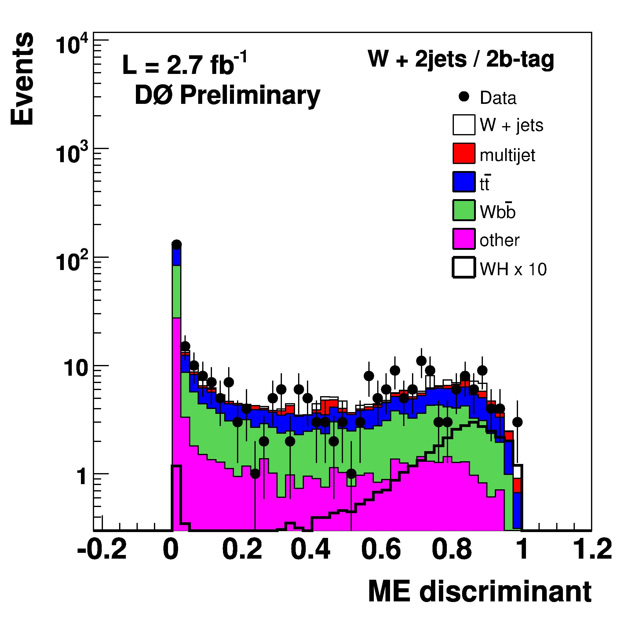
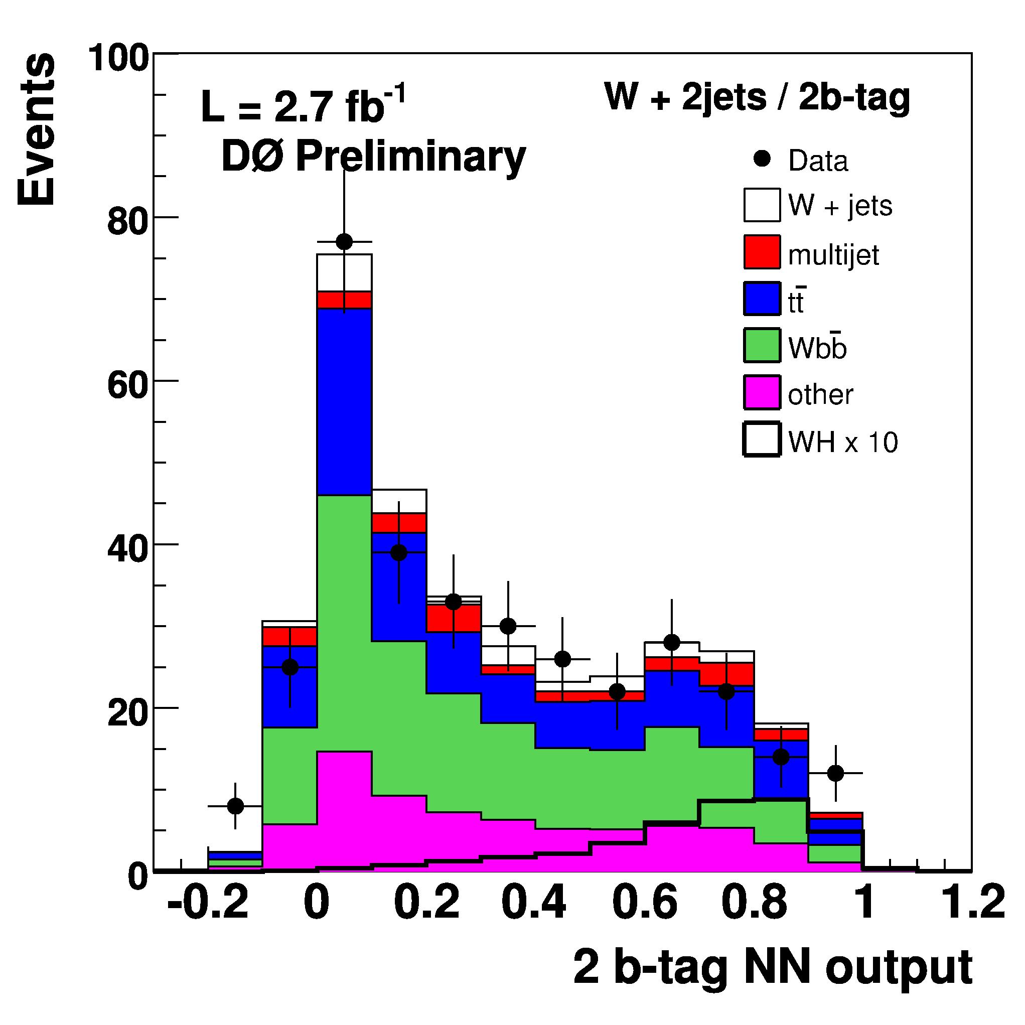
Apart from b-tags, the signal displays a different kinematics than all backgrounds. Again, seven variables are used, which now describe the event kinematics: the transverse energy of the second-leading jet, the angle between jets, the dijet invariant mass, and a matrix-element discriminant, which is computed by comparing the probability density of the quadrimomenta of the objects produced in the decay in a WH event to that of backgrounds. In the figure above, the matrix element discriminant is shown for all the processes contributing to the class of W+2jet events with two b-tags. The output of the neural network shows that Higgs events fall in the right-side of the distribution, while backgrounds pile up mostly on the left, as can be seen in the figure below.
Results of the search
Since no signal is observed in the NN output distribution seen in the data, DZERO proceeds to set upper limits on the signal cross-section. For 2-jet events they use the NN output is used, while they use the dijet mass distribution for the 3-jet event classes. No justification is provided in their paper for this choice, which looks slightly odd to me, but I imagine they have done some optimization studies before taking this decision. However, I would imagine that the NN output is in principle always more discriminant than just one of the variables on which the network is constructed… Maybe somebody from DZERO could clarify this point in the comments thread, to the benefit of the other readers ?
At the end of the day, DZERO obtains limits on the cross section of the searched signal, which are still above the standard model predictions whatever the Higgs mass: therefore, they do not provide an exclusion of mass values, yet. These results, however, once combined with other results from CDF and DZERO, will one day directly imply that a SM Higgs cannot exist, if its mass is in a specified range. In the graph below you can see the limit set by this analysis on the WH production cross-section as a function of Higgs mass.
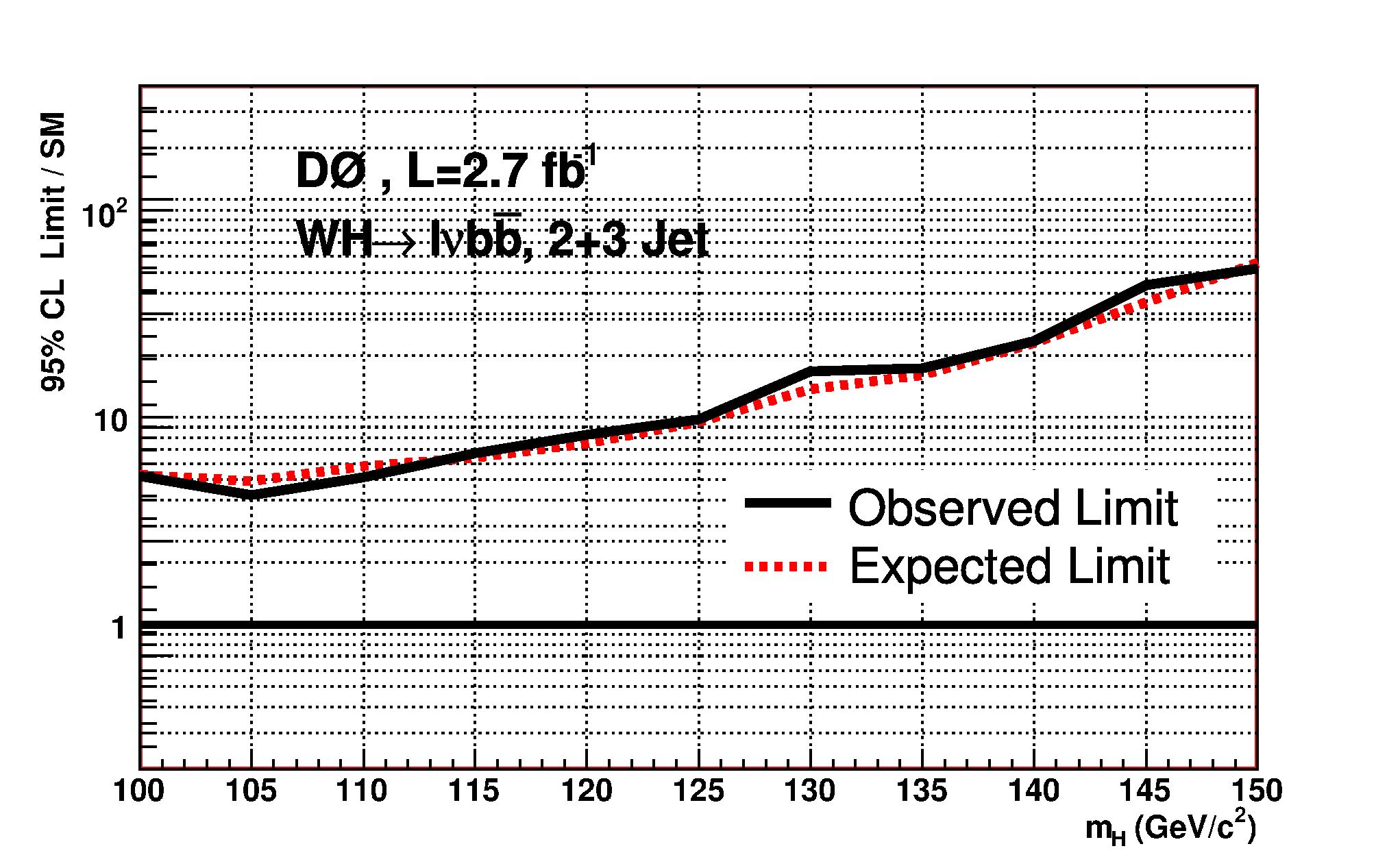
The black curve shows the 95% exclusion, while the hatched red curve shows the result that DZERO was expecting to find, based on pseudoexperiments. The comparison of the two curves is not terribly informative, but it does show that there were not surprises from the data.

The result can also be shown in the standard “LLR plot” above, which is showing, again as a function of the Higgs boson mass, the log-likelihood ratio of two hypotheses: the “background only” and the “signal+background” one. Let me explain what that is. For each mass value on the x-axis, imagine the Higgs is there. Then, with large statistics, the data would show a propension for the “signal plus background” hypothesis, and the LLR would be large and negative. If, instead, the Higgs did not exist at any mass value, the LLR would be large and positive. The two hypotheses can be run on pseudo-data of the same statistical power as the data really collected, thus producing the red and black hatched lines in the plot below. The two curves are different, but the red one does not manage to depart from the green band constructed around the black hatched one: that means that the data size and the algorithms used in the analysis do not have enough power to discriminate the two hypotheses, not even at 1-sigma level (which is the meaning of the width of the green band, while the yellow one shows two-sigma contours). The full black line shows the behavior of real data: they have a propension of confirming the background-only hypothesis at low mass, and a slight penchant for the signal+background one at about 130 GeV. But this is a really, really small fluctuation, well within the one-sigma band!
I think the LLR plot is a great way to describe the results of the search visually. It at once tells you the power of the analysis and the available data, and the outcome on the real events collected. Now, it takes twenty thick lines of text to explain it, but once you’ve grabbed its meaning…
