Zooming in on the Higgs March 24, 2009
Posted by dorigo in news, physics, science.Tags: CDF, DZERO, Higgs boson, LEP, MSSM, standard model, supersymmetry, Tevatron, top quark, W boson
trackback
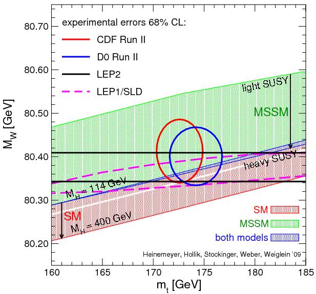 Yesterday Sven Heinemeyer kindly provided me with an updated version of a plot which best describes the experimental constraints on the Higgs boson mass, coming from electroweak observables measured at LEP and SLD, and from the most recent measurements of W boson and top quark masses. It is shown on the right (click to get the full-sized version).
The graph is a quite busy one, but I will try below to explain everything one bit at a time, hoping I keep things simple enough that a non-physicist can understand it.
The axes show suitable ranges of values of the top quark mass (varying on the horizontal axis) and of the W boson masses (on the vertical axis). The value of these quantities is functionally dependent (because of quantum effects connected to the propagation of the particles and their interaction with the Higgs field) on the Higgs boson mass.
The dependence, however, is really “soft”: if you were to double the Higgs mass by a factor of two from its true value, the effect on top and W masses would be only of the order of 1% or less. Because of that, only recently have the determinations of top quark and W boson masses started to provide meaningful inputs for a guess of the mass of the Higgs.
Top mass and W mass measurements are plotted in the graphs in the form of ellipses encompassing the most likely values: their size is such that the true masses should lie within their boundaries, 68% of the time. The red ellipse shows CDF results, and the blue one shows DZERO results.
 There is a third measurement of the W mass shown in the plot: it is displayed as a horizontal band limited by two black lines, and it comes from the LEP II measurements. The band also encompasses the 68% most likely W masses, as ellipses do.
In addition to W and top masses, other experimental results constrain the mass of top, W, and Higgs boson. The most stringent of these results are those coming from the LEP experiment at CERN, from detailed analysis of electroweak interactions studied in the production of Z bosons. A wide band crossing the graph from left to right, with a small tilt, encompasses the most likely region for top and W masses.
 So far we have described measurements. Then, there are two different physical models one should consider in order to link those measurements to the Higgs mass. The first one is the Standard Model: it dictates precisely the inter-dependence of all the parameters mentioned above. Because of the precise SM predictions, for any choice of the Higgs boson mass one can draw a curve in the top mass versus W mass plane. However, in the graph a full band is hatched instead. This correspond to allowing the Higgs boson mass to vary from a minimum of 114 GeV to 400 GeV. 114 GeV is the lower limit on the Higgs boson mass found by the LEP II experiments in their direct searches, using electron-positron collisions; while 400 GeV is just a reference value.
The boundaries of the red region show the functional dependence of Higgs mass on top and W masses: an increase of top mass, for fixed W mass, results in an increase of the Higgs mass, as is clear by starting from the 114 GeV upper boundary of the red region, since one then would move into the region, to higher Higgs masses. On the contrary, for a fixed top mass, an increase in W boson mass results in a decrease of the Higgs mass predicted by the Standard Model. Also note that the red region includes a narrow band which has been left white: it is the region corresponding to Higgs masses varying between 160 and 170 GeV, the masses that direct searches at the Tevatron have excluded at 95% confidence level.
 The second area, hatched in green, is not showing a single model predictions, but rather a range of values allowed by varying arbitrarily many of the parameters describing the supersymmetric extension of the SM called “MSSM”, its “minimal” extension. Even in the minimal extension there are about a hundred additional parameters introduced in the theory, and the values of a few of those modify the interconnection between top mass and W mass in a way that makes direct functional dependencies in the graph impossible to draw. Still, the hatched green region shows a “possible range of values” of the top quark and W boson masses. The arrow pointing down only describes what is expected for W and top masses if the mass of supersymmetric particles is increased from values barely above present exclusion limits to very high values.
So, to summarize, what to get from the plot ? I think the graph describes many things in one single package, and it is not easy to get the right message from it alone. Here is a short commentary, in bits.
- All experimental results are consistent with each other (but here, I should add, a result from NuTeV which finds indirectly the W mass from the measured ratio of neutral current and charged current neutrino interactions is not shown);
- Results point to a small patch of the plane, consistent with a light Higgs boson if the Standard Model holds
- The lower part of the MSSM allowed region is favored, pointing to heavy supersymmetric particles if that theory holds
- Among experimental determinations, the most constraining are those of the top mass; but once the top mass is known to within a few GeV, it is the W mass the one which tells us more about the unknown mass of the Higgs boson
- One point to note when comparing measurements from LEP II and the Tevatron experiments: when one draws a 2-D ellipse of 68% contour, this compares unfavourably to a band, which encompasses the same probability in a 1-D distribution. This is clear if one compares the actual measurements: CDF
(with 200/pb of data), DZERO
(with five times more statistics), LEP II
(average of four experiments). The ellipses look like they are half as precise as the black band, while they are actually only 30-40% worse. If the above is obscure to you, a simple graphical explanation is provided here.
- When averaged, CDF and DZERO will actually beat the LEP II precision measurement -and they are sitting on 25 times more data (CDF) or 5 times more (DZERO).
Comments
Sorry comments are closed for this entry

Note that with SM and MSSM treated as two and only, a priori possible, equally likely alternatives, the Tevatron measurements say that MSSM is true with 80+ percent probability.
Well, the SUSY particles are not that heavy. The centers of the CDF/D0 circles are actually closer to the central axis of the MSSM strip than to its boundary. Especially your CDF circle is supersymmetric enough. 😉
The superpartner masses at the point are comparable to 200 GeV, aren’t they? We’re not talking about new particles above many TeVs, are we?
Finally, may I ask a really elementary question? Why are the three masses linked at all? There are many independent couplings and parameters to dictate them – the Higgs vev; the electroweak couplings (the previous 2 give the W mass); the quartic coupling (in front of the Higgs mass); the top Yukawa coupling (in front of the top mass).
What is the known relationship between the parameters above that you use and I am not seeing?
Any idea how heavy ?
Is there any reason why the CDF analysis is so old to have used only 0.2 fb-1? Just a matter of priorities?
Lubos,
I’m no expert in these measurements, but I assume the link is the following:
M_W = \frac{1}{2}gv
where g is SU(2) coupling, and v the Higgs VEV
Top mass = \frac{Y_t v}{\sqrt{2}}
putting v in terms of M_W gives:
= \sqrt{2}\frac{Y_t M_W}{g}
where Y_t the top Yukawa couplig
Higgs mass – constrains v (M_H = v\sqrt{2\lambda})
So they are all linked by g (SU(2) coupling) and v (Higgs VEV) through the W mass.
@JJ
no, this is more complicated. As you can see from your last formula, the Higgs mass is an independent parameter (since lambda is independent of g and v)
The W-boson mass (and the top mass?) depend on the Higgs mass through radiative corrections.
More precicely (and maybe wrong):
Take the Higgs vev v fixed, then this predicts the W mass quite accurately at the tree level. Now the top mass is still a free parameter via the top-yukawa coupling, Y_t in your formula. Top quark loops give a correction to the W-boson mass at the 1-loop level, thus introducing a dependence of the W-mass on the top mass. This gives the upward slope in the green and red bands. Now additionally there are the corrections from the Higgs loops, although they are much weaker. As the Higgs mass increases, the W-mass goes down (very slowly), et voila, you get the red band for the SM (the one for Susy might be a bit more complicated to obtain).
Some details might be wrong in the last paragraph since I don’t know how these plots are actually done.
Cheers.
Dear JJ #4, thanks for your attempt, although I apologize for agreeing with the criticism in #5.
Dear anonymous #5, thanks even more for your attempt 😉 but I still don’t understand how the measurement distinguishes the part of the W mass from the loop corrections.
There are probably several independent measurements of it (or the vev), right? 😉 And their difference must kind of inform us about the loop corrections more directly.
Some more explanations for those who are interested:
1) Within the SM the three quantities M_W, m_t and M_H are linked by
radiative corrections (as explained by anonymous 5). To see it in a simple picture: the W-self-energy (which somehow determines its mass) receives loop-corrections, e.g. from a top-bottom loop or from a W-Higgs loop. In this way one finds M_W(m_t, M_H). It turns out that the corrections to M_W go at leading order like m_t^2 and like log(M_H). Consequently, the dependence on m_t is much stronger than on M_H.
BTW: this correlation was used to predict the top quark mass successfully several years before the direct discovey.
2) Within the MSSM one can calculate M_W in a similar way. The differences to the SM calculation are: a) SUSY particles enter in the loops (where the most prominent role is played by the scalar tops and bottoms), b) the Higgs boson masses (exept of one free mass scale) are not free parameters anymore, but depend on the SUSY masses. This is especially true for the lightest MSSM Higgs mass, which usually contributes in a similar way as the SM Higgs.
The scalar top and bottom corrections always give a positive contribution to M_W, and therefore one finds M_W(MSSM) > M_W(SM) as can be seen in the plot.
3) M_W alone is not sufficient to determine the various SUSY mass scales that contribute here. M_W only cuts out one hyper-dimensional slice of the MSSM parameter space. Consequently, the M_W-m_t measurement is compatible with relatively light scalar tops, but also with heavier ones. In general one can say that scalar top masses around 500 GeV fit quite well.
4) If one really wants to determine some masses one should go to simplified models (such as the CMSSM/mSUGRA, GMSB, AMSB, …) and include more constraints. This issue was discussed in this blog several months ago. 🙂
Dear Sven #7, thanks but let me ask more explicitly once again. Could you please explain how can one disentangle the tree-level contributions to the W mass from the radiative corrections?
How do you know that the deviations found for the W mass are telling us about different loop corrections rather than a different tree-level starting value?
I suppose that the “SM Higgs vev” is determined at least in two different ways, one of which being the W mass measurement. But what are the actual measurements that are used to reconstruct the otherwise unknown relationship between mTop, mW, and mHiggs?
This is a very confusing plot (although it’s not the first time I see it circulated). The only general statement I would make is that MSSM fares no worse and no better than the light-higgs SM with respect to the electroweak precision tests. It’s not fair to say that the EWPT are capable to distinguish between the two.
A question to Tommaso: do you know by any chance what is the systematic/statistical splitting of the Tevatron W mass measurement error?
Dear Lubos,
one does not disentangle tree-level from corrections, the whole point of comparing theory and experiment is to derive relations between physical observables (e.g. pole masses) and check if the experiments confirm these relations. Let’s stick for example to the SM case. You can write a relation between the SM physical observables:
G_mu/Sqrt(2) = Pi alpha_em/2/sw^2/mw^2 (1+delta)
Where G_mu is the muon decay constant, alpha_em is the fine structure constant, sw^2 is just a placemat for 1-mw^2/mz^2 and delta is the radiative correction, a perturbatively calculable function of the SM observables (including the not-so-well measured mt and the unmeasured mH).
Then you can invert that formula and get a prediction for mw as a function of all the other parameters. For any given value of mt and mH, this relation will identify a point in the plane corresponding to the “SM” expectation for mw. Then you just check how well that point falls in the ellipses from the Tevatron measurements. If it falls too much outside the ellipse it means that the value of mH you started from is not compatible with the top mass measurement and with the SM prediction for mw (of course you could as well swap the roles of mt and mw and do the same reasoning).
I hope this helps, otherwise you can always check the literature for the technicalities: http://pdg.lbl.gov/2008/reviews/rpp2008-rev-standard-model.pdf
Cheers Ptrslv72
sorry, just a quick correction: you could *not* swap the roles of mt and mw and do the same reasoning, because mt enters the relation above only at loop level (i.e. in the delta). Cheers Ptrslv72
Dear Ptrslv72, indeed, the statement that it makes no physical sense to try to separate tree-level terms from the corrections was the whole point of my previous complaints #6 and #8 above, so it would have been more honest if you didn’t try to revert my point completely. 😉
Fine, thanks, so you’re saying that the Higgs vev is measured from the muon decay constant. A strange choice. Still, this trick depends on the assumption that different but similar quantities – like m(W) and G(mu) – are influenced differently by the loop corrections.
Am I wrong in reading this chart that, if the current estimates of the mass of the W and T are accurate (80.39 +- 0.025 and 173.1 +- 1.3), that the standard model Higgs is excluded by LEP II? (To the 95% confidence limit of the LEP II result.)
Also – I find the pink and blue elipses (68%? Why?) rather confusing — don’t both CDF and D0 claim to have more accurate measurements of both W and T masses?
Surely I’m missing something.
Dear Lubos, Ptrslv72,
most was explained already by Ptrslv72. One could add that the tree-level
value of M_W in the SM and the MSSM are the same, therefore any difference in this case can be attributed to the loop corrections.
Dear Slava,
it is correct that the SM cannot be ruled out by electroweak precision data
((g-2)_mu could lead to a long discussion though). However, if one combines all measurements shown in the plot, the 68% C.L. ellipse lies nearly entirely in the MSSM area, i.e. the MSSM is *slightly* favored by the combination of M_W and m_t. You can check out the plots on the web page linked at the very top of this page.
Sorry Lubos I did not mean to make you look like a clueless string theorist 😉 This said, I don’t fully understand your last comment. The correction term “delta” in the relation that I wrote above is the combination of different contributions, i.e. the various corrections to the tree-level relations between the physical observables G_mu, alpha_em, mZ and mW the underlying Lagrangian parameters v (the Higgs vev), g and g’ (the gauge couplings). The fact that these corrections differ from each other is not an assumption, it is the result of a calculation. E.g. you can easily convince yourself that the correction to G_mu depends on the W self-energy computed at
zero external momentum while the correction to mw depends on the W self-energy computed at the W pole. Cheers Ptrslv72
Dear Sven,
you are talking about one sigma effects, it’s squeezing water out of stone, that’s why I think the plot is misleading. For instance, it misled Motl to say above that susy is 80% right, which is ridiculous.
The correct statement is that susy, being a weakly coupled SM extension, is simply not usefully discriminateable from it on the basis of the EWPT (and becomes indistinguishable from it in the decoupling limit). Strongly coupled extensions like Higgsless models or composite Higgs, it’s a different story.
Best, Slava
Aha interesting. I was concerned about the lambda, and figured it could either be argued away (in which case someone would explain), or that my reasoning was wrong (in which case someone would explain)!
Hi Tommaso,
This comment is more about the unified theory, than the Higgs.
I have become fascinated with Eugenio Beltrami, an Italian mathematician, who in 1888 apparently unified electomagnetism with mechanics.
TW Barrett and DM Grimes edited Advanced Electromagneism: Foundations, Theory and Applications, World Scientific, 1995, searchable on Google books.
This book has 3particlarly interesting chapters:
ch 2 Helicity and EM field theory
ch 7 Foundational electrodynamics and Beltrami vector fields
ch 10 Gravitation as a 4th order effect.
Is this a key to the theory of everything [TOE] ?
Beltrami flow is used in medical imaging, hydrodynamics and dynamos.
Dear Sven and PtrSlv,
so far none of you has answered my question what is the relationship between mW, mTop, mHiggs that is used in the graphs, and what are the other independently (and more accurately) measured quantities that make this relationship possible.
You’re just bullshiting about other relationships that might be “similar”. I am not interested in other relationships here and I am not interested in arrogant commenters who say that they understand something if they obviously don’t.
Slava #16, I made a rather accurate statement (about those 80%) and the statement directly and tautologically follows from my assumptions, the rules of the game that were properly and fully explained, and Tommaso’s graph. (For example, “Higgsless models” were eliminated at the very beginning, and for good reasons.) On the other hand, your “not usefully discriminateable” answer is just spreading a biased, unquantitative fog.
Best wishes
Lubos
Dear Slava Rychkov #16,
let me be a bit more detailed in the description why: if you think that the first graph Tommaso posted above doesn’t imply that assuming 50:50 priors for SM and MSSM, the probability of MSSM is 80-90 percent, then you are reading the graph incorrectly.
Take e.g. the CDF ellipse. It shows the peak of a probability distribution for the values that they measure. Imagine it is a normal distribution, which it essentially is. The ellipse includes regions whose overall probability is, according to CDF, 68%. Among those 68%, about 90% (of the ellipse) is in the MSSM region, and implies that SM is excluded and MSSM must hold (by the assumption of 2 theories).
Outside the ellipse, which is 32% of the distribution, the percentage of the SM region is about 30% of the overall probability while MSSM is 70% or so. Taking the weighted average, you get over 80% for MSSM. For D0, it is analogous, but slightly less, so I say that the CDF/D0 combined figure is about 80%.
This is nothing else than Bayesian inference. 80% is not any kind of “certainty” but it is higher than 50%, and this conclusion about “higher than 50% odds” can be derived from 1-sigma statistical results like this one, and you’re just wrong if you think otherwise.
Actually, if one combined the CDF/D0 ellipses on the graph, the area of the ellipse in the graph would shrink 2 times or sqrt(2) times – I don’t want to think too much now. A 1-sigma signal would become a sqrt(2)-sigma signal or so, and I would get closer from 80% towards 100%.
It is within the reach of the Tevatron-like collider to sharpen this precision measurement to the extent that it would pretty much exclude SM in favor of the MSSM-like alternatives. They’re arguably beginning to do such a thing. Your statement that SM and MSSM couldn’t be discriminated by such tests is simply wrong. It would be only correct assuming that Nature likes to stay in the decoupling limit, or very massive superpartners etc.
But the most preferred figures in the graph suggest otherwise. The most likely points indicate that Nature likes to be close to the center of the MSSM region – so it may be a garden-variety MSSM-like model. It is not true that SM and MSSM are indistinguishable assuming generic assumptions about them. And it is also untrue that MSSM gives an infinitely higher uncertainty about everything because of its unknown soft-SUSY breaking terms. The graph above shows that the uncertainty of things – like the relation between mW and mTOP – in “most of” MSSM is comparable to that of the Standard Model, at most 2 times broader.
Even when it comes to similar dirty phenomenology, MSSM is a damn robust model. Because of these phenomenological observations and especially because of deeper theoretical reasons, it’s simply wrong to consider MSSM as a random subclass of beyond-the-SM models. It is a very special class whose prior probabilities should always be taken close to those of the Standard Model itself.
Let me also translate the adjective “usefully discriminateable” that you used. It sounds positive, doesn’t it? But you know what this word means? It means “essentially excluded”. If something is “usefully discriminateable” by similar graphs like Tommaso’s first graph, more so than MSSM, then it is simply falsified, at a pretty high confidence level – because most of the corresponding ellipse would be far from the measured values. I don’t think that a completely sane person would view such a property as an advantage of a theory.
Best wishes
Lubos
Dear Lubos
first learn some basics of the EWPT. then we talk.
Best, Slava
ooooh, here comes the real Lubos Motl, arrogant and gratuitously insulting. The previous, kinder one must have been an impostor… 😉
What do you want, that we write down in a blog the explicit formulae for the dependence of the correction to mW on mt and on mH? Several people already wrote that it is quadratic on the former and logarithmic on the latter. Then you are a physicist, you should be able to check the literature by yourself for the details. If you want to start putting in practice Slava’s suggestion (to which I subscribe) you can start from hep-ph/0512342. Cheers Ptrslv72
Hi all,
well, I leave this thread for an evening and I find 20 messages to deal with… I thank those who contributed with answers to the few questions that were posed above, but let me go through the comments and make a few points.
1) and others) Lubos, you should not let go with such eyeballing estimates. Many here have tried to explain that the MSSM is just as uncomfortable with a high Higgs boson mass as the SM is: that is, the experimental situation nowadays sees a lower limit at 114 GeV, plus a global EW fit (which includes top and W mass measurements) which points to a lower central value. The combined effect of these is to leave a narrow region of likely masses for the lightest scalar in the MSSM as well as for the SM-proper higgs.
In other words, you should not just rely on W mass measurements (the only ones which appear to “discriminate” between SM and MSSM in the plot) to draw conclusions, but also on the 114 GeV LEP II limit. Taken together, the two inputs leave both the SM and the MSSM a bit dissatisfied, but the “phase space” of the two is largely equivalent, in the assumption that the MSSM extension does not alter global fits enough to change the answer.
I will post later today a plot that combines all information. From it, and from some older plots which Sven Heinemeyer himself produced in a paper of last year, you can make up your mind on whether your 80% makes sense or not.
2) Sumar, I think you should refer to Sven’s answers above, particularly #7. I think the model parameters are too many to allow a precise answer, though.
3) Andrea, the reason why CDF only published 200/pb (two years ago), is that the W mass analysis is -IMHO- THE most difficult analysis that the Tevatron experiments perform nowadays. It involves calibrations of tracker and calorimeter to fractions of a permille, horribly complicated checks of all kinds, huge MC statistics, additional side measurements (of PDF through W asymmetry distributions, for instance), study of material in the tracker, etcetera, etcetera. CDF is working at a 2/fb measurement if I understand things correctly, but it will take a while longer. When it will be out, it will be the most precise single measurement in the world, I believe.
9) Hi Slava, I can give you these figures: ;
; .
.
CDF:
DZERO:
These are only the latest measurements, based on 200/pb and 1000/pb, respectively; the first uncertainty is statistical. You can well see that CDF has the smallest systematics, even though they only studied a fifth of the data. Already by not doing anything smarter for systematics and just scaling by statistics, a 1/fb measurement by CDF should get a reduction of the statistical error from 34 to 15 MeV, with the result that the total error might end up being in the 37 MeV ballpark with 1/fb, so significantly smaller than the 44 MeV total error of DZERO with an equivalent dataset.
Once past Tevatron measurements are averaged with the two above, the Tevatron average is predicted to already have a better precision than the LEP II one. But I think that the data that CDF and DZERO have collected will eventually result in a combined W mass measurement with uncertainty well below 20 MeV, possibly below 15.
13) Amos, no, I think you cannot say that. The LEP EWWG quotes after a global fit including all measurements.
18) Doug, I haven’t a clue!
20) Lubos, I think you should not ignore part of the experimental data. LEP II excluded masses below 114 GeV, and you should put this together with the “ellipses”.
Cheers all,
T.
PS I think it is time I present some of the most updated results on global fits in a separate post… Will do today if I have a chance.
Euclid and Newton are incomplete (parallel lines; c and h) . No axiomatic system is stronger than its weakest axiom. So too the Higgs, SUSY, SUGRA, string theory, QFT, and general relativity – but only if prior observations remain valid! Perhaps the vacuum has a chiral anisotropic pseudoscalar background only active in the massed sector. Cosmic inflation, matter vs. antimatter abundance, and biological homochirality then have a common origin. Nobody has challenged the vacuum with chemically identical, opposite parity mass configurations, for physics eschews chemistry.
Einstein’s elevator would fail for left and right shoes. Anisotropic vacuum plus Noether’s theorem selectively ends conservation of angular momentum, impacting QFT. Perturbative string theory, demanding BRST invariance uniting the effects of a massive body and inertial acceleration, is gone. SUGRA has no basis. SUSY is in trouble. The Higgs, strongly coupled to a chiral Weak interaction vector boson, is less well defined.
Nature kindly provides homochiral 3-fold atomic helices in kilogram self-similar aggregates – enantiomorphic crystallographic space groups P3(1)21 (right-handed helices) and P3(2)21 (left-handed helices). There are no racemic or conflicting screw axes therein. The opposite shoes are grown as quartz, cinnabar, berlinite and analogues, tellurium, selenium… Run a parity Eötvös experiment opposing single crystal test masses of cultured left- and right-handed quartz, 0.304 nm diameter sphere chirality emergence scale. Amorphous fused silica is the control sock against each shoe.
Contemporary physics could have a detectably weak founding postulate. A parity Eötvös experiment runs in 90 days using commercial materials in existing apparatus with validated protocols. Somebody should look.
Dear Tommaso,
thanks for giving a breaking of the experimental error in mW measurement. What is the rule for combining systematic errors when the measurements are combined? I guess that some, and maybe even a large, part of the systematic error must be of theoretical origin, i.e. the same in the D0 and Tevatron measurement. That part cannot be reduced via simple combination of measurements. So I find eventual 15 MeV error a tall order. But I will be glad to be proved wrong.
Hi Slava,
systematic uncertainties decrease with luminosity too, albeit not all with a square root law. For instance, momentum and energy scale systematics actually does follow a square root law, because it is driven by the statistics of the resonances used to calibrate those measurements. On the other hand, the systematics which scale less with luminosity are the PDF, which are in principle independent on it. In practice, though, a measurement of the W production asymmetry by the Tevatron experiments can reduce those too. If you look at the current DZERO measurement, their total systematic uncertainty is dominated by the energy scale. Theoretical uncertainties are three times smaller, 12 MeV total. Check in Table II of their paper here.
The CDF collaboration will soon publish a W mass measurement based on 2.3/fb of data. With it, we already know that the statistical uncertainty will be of 16 MeV. I expect that the systematic error will be of the order of 20-25 MeV. Check this page for details.
Cheers,
T.
Thanks Tommaso, very clear.